
rm(list = ls())
library("ggplot2")Software
We use the statistical software environment R (R Core Team, 2024), and R add-on packages ggplot2 (Wickham, 2016).
This document is produced using Quarto (Allaire et al., 2024).
Organize R Session
Linear Regression Model
Data Simulation
Data are simulated according to the equations given in the lecture slides1:
set.seed(123)
N <- 500
df <- data.frame(x_1 = runif(n = N),
                 x_2 = runif(n = N))
(beta_0 <- rnorm(n = 1, mean = 1, sd = .1))
[1] 0.9398107(beta_x_1 <- rnorm(n = 1, mean = 1, sd = .1))[1] 0.9006301(beta_x_2 <- rnorm(n = 1, mean = -.5, sd = .1))[1] -0.3973215(sigma <- rgamma(n = 1, shape = 1, rate = 4))[1] 0.293026df$mu <- beta_0 + beta_x_1 * df$x_1 + beta_x_2 * df$x_2
df$y <- df$mu + rnorm(n = N, mean = 0, sd = sigma)Visualisations
ggplot(data = df, aes(x = x_1, y = x_2)) +
  geom_point()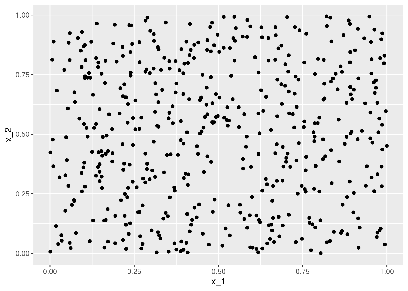
x_1 and x_2 - each from the uniform distribution between \(0\) and \(1\).
ggplot(data = df, aes(x = x_1, y = mu, color = x_2)) +
  geom_point()
x_1 with response y - each individual observation is coloured according to the second covariate x_2.
ggplot(data = df, aes(x = x_2, y = mu, color = x_1)) +
  geom_point()
x_2 with response y - each individual observation is coloured according to the first covariate x_1.
ggplot(data = df, aes(x = x_1, y = x_2, color = mu)) +
  geom_point()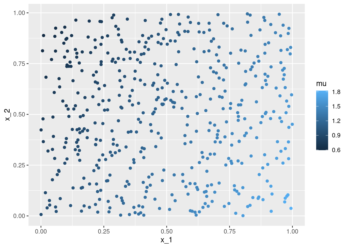
x_1 and x_2 - each individual observation is coloured according to the underlying true conditional expectation mu.
ggplot(data = df, aes(x = x_1, y = x_2, color = y)) +
  geom_point()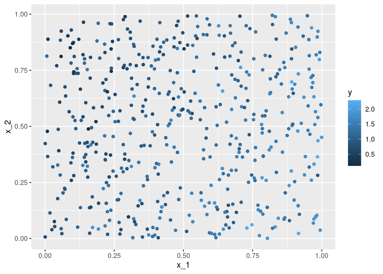
x_1 and x_2 - each individual observation is coloured according to the response y.
Modeling
The basic R command for (frequentist) estimation of the parameters of a linear regression model is a call to the function lm:
Call:
lm(formula = y ~ x_1 + x_2, data = df)

Residuals:
     Min       1Q   Median       3Q      Max
-0.82082 -0.19805  0.00329  0.19051  0.81138

Coefficients:
            Estimate Std. Error t value Pr(>|t|)
(Intercept)  0.91291    0.03448  26.476  < 2e-16 ***
x_1          0.91533    0.04668  19.610  < 2e-16 ***
x_2         -0.36218    0.04566  -7.933 1.43e-14 ***
---
Signif. codes:  0 '***' 0.001 '**' 0.01 '*' 0.05 '.' 0.1 ' ' 1

Residual standard error: 0.2963 on 497 degrees of freedom
Multiple R-squared:  0.4674,    Adjusted R-squared:  0.4652
F-statistic:   218 on 2 and 497 DF,  p-value: < 2.2e-16
Visualisations
nd <- data.frame(x_1 = seq(0, 1, by = .1),
                 x_2 = .5)
nd$mu <- predict(m, newdata = nd)
ggplot(data = df, aes(x = x_1, y = mu, color = x_2)) +
  geom_point() +
  geom_line(data = nd, aes(x = x_1, y = mu, color = x_2))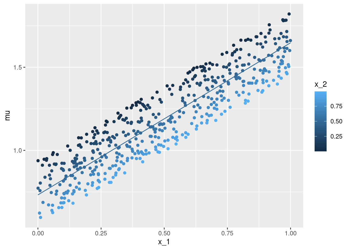
x_1 with the true conditional expectation mu - each individual observation is coloured according to the second covariate x_2. The line gives the point estimation for the conditional expectation with the second covariate x_2 fixed to \(0.5\).
nd <- data.frame(expand.grid('x_1' = seq(0, 1, by = .1),
                             'x_2' = seq(0, 1, by = .1)))
nd$mu <- predict(m, newdata = nd)
ggplot(data = df, aes(x = x_1, y = mu, color = x_2)) +
  geom_point() +
  geom_line(data = nd, aes(x = x_1, y = mu, color = x_2, group = x_2))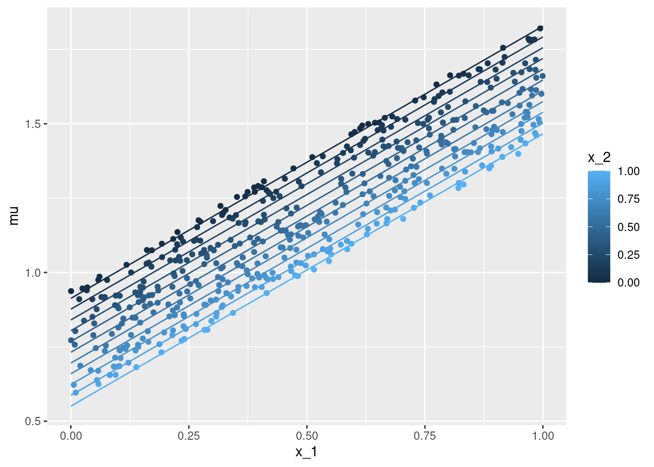
x_1 with the true conditional expectation mu - each individual observation is coloured according to the second covariate x_2. The lines give the point estimation for the conditional expectation with the second covariate x_2 taking on values between \(0\) and \(1\) (at steps of \(0.1\)).
Add-Ons
Add-On Linear Model: A) Stancode
Stan Users Guide
Probabilistic Programming Languages such as Stan (Carpenter et al., 2017) allow to plug together the single parts of a statistical regression model2:
The following Stan-code is published here in the Stan users guide:
data {
  int<lower=0> N;
  vector[N] x;
  vector[N] y;
}
parameters {
  real alpha;
  real beta;
  real<lower=0> sigma;
}
model {
  y ~ normal(alpha + beta * x, sigma);
}
Stancode generated by calling brms::brm
The R add-on package brms (Bürkner, 2017, 2018) allows to implent advanced regression models without being an expert in ‘Stan-programming’.
Here is the Stan-code that is implemented by ‘brms’ for our linear regression model example:
brms::make_stancode(brms::bf(y ~ x_1 + x_2, center = F), data = df)// generated with brms 2.21.0
functions {
}
data {
int<lower=1> N; // total number of observations
vector[N] Y; // response variable
int<lower=1> K; // number of population-level effects
matrix[N, K] X; // population-level design matrix
int prior_only; // should the likelihood be ignored?
}
transformed data {
}
parameters {
vector[K] b; // regression coefficients
real<lower=0> sigma; // dispersion parameter
}
transformed parameters {
real lprior = 0; // prior contributions to the log posterior
lprior += student_t_lpdf(sigma | 3, 0, 2.5)
- 1 * student_t_lccdf(0 | 3, 0, 2.5);
}
model {
// likelihood including constants
if (!prior_only) {
target += normal_id_glm_lpdf(Y | X, 0, b, sigma);
}
// priors including constants
target += lprior;
}
generated quantities {
}Add-On Linear Model: B) Posterior predictive check: an introduction ‘by hand’
Having an lm object already, it is rather straightforward to get posterior samples by using function sim from the arm (Gelman & Su, 2024) package:
library("arm")S <- sim(m)
str(S)Formal class 'sim' [package "arm"] with 2 slots
..@ coef : num [1:100, 1:3] 0.882 1.014 0.904 0.978 0.958 ...
.. ..- attr(*, "dimnames")=List of 2
.. .. ..$ : NULL
.. .. ..$ : chr [1:3] "(Intercept)" "x_1" "x_2"
..@ sigma: num [1:100] 0.323 0.303 0.292 0.309 0.29 ...S <- cbind(S@coef, 'sigma' = S@sigma)
head(S) (Intercept) x_1 x_2 sigma
[1,] 0.8816414 0.9245094 -0.3362733 0.3227662
[2,] 1.0139849 0.7317948 -0.3398411 0.3033703
[3,] 0.9037042 0.9155575 -0.3506924 0.2922883
[4,] 0.9776909 0.8392790 -0.3845609 0.3090220
[5,] 0.9579213 0.8977625 -0.4284596 0.2900632
[6,] 0.9549211 0.8478278 -0.3937226 0.3094227Predict the response for the covariate data as provided by the original data-frame df - here only by using the first posterior sample:
s <- 1
S[s, ]
(Intercept) x_1 x_2 sigma
0.8816414 0.9245094 -0.3362733 0.3227662 mu_s <- S[s, '(Intercept)'] + S[s, 'x_1'] * df$x_1 + S[s, 'x_2'] * df$x_2
y_s <- rnorm(n = nrow(df), mean = mu_s, sd = S[s, 'sigma'])
pp <- rbind(data.frame(y = df$y, source = "original", s = s),
data.frame(y = y_s, source = "predicted", s = s))
ggplot(data = pp, aes(x = y, fill = source)) +
geom_histogram(alpha = .5, position = "identity")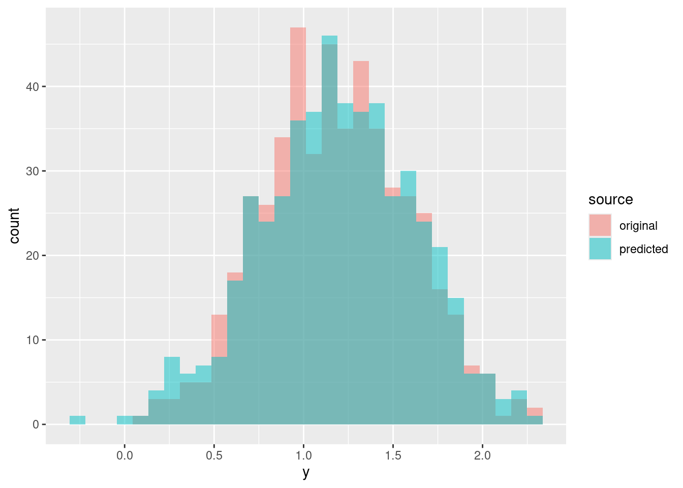
Now let’s repeat the same for 9 different posterior samples:
pp <- NULL
for (s in 1:9) {
  mu_s <- S[s, '(Intercept)'] + S[s, 'x_1'] * df$x_1 + S[s, 'x_2'] * df$x_2
  y_s <- rnorm(n = nrow(df), mean = mu_s, sd = S[s, 'sigma'])
  pp <- rbind(pp,
              data.frame(y = df$y, source = "original", s = s),
              data.frame(y = y_s, source = "predicted", s = s))
}
ggplot(data = pp, aes(x = y, fill = source)) +
  geom_histogram(alpha = .5, position = "identity") +
  facet_wrap(~ s)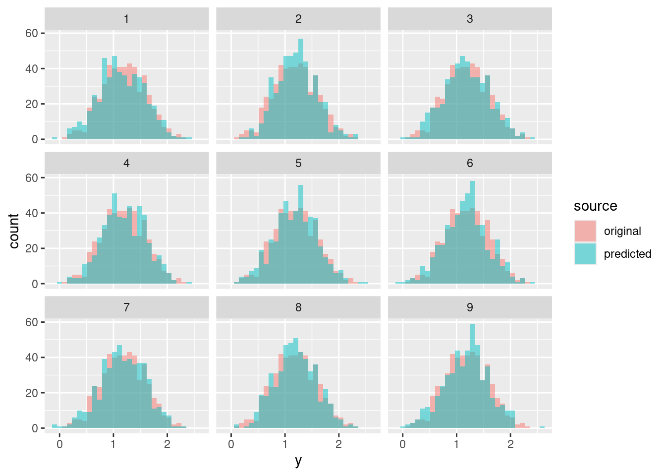
ggplot(data = pp, aes(x = y, fill = source)) +
  geom_density(alpha = .5, position = "identity") +
  facet_wrap(~ s)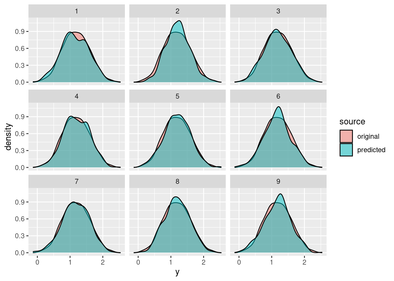
ggplot(data = pp, aes(x = y, colour = source)) +
  stat_ecdf() +
  facet_wrap(~ s)
ggplot(data = subset(pp, source == "predicted"),
       aes(x = y, group = s)) +
  geom_density(position = "identity", fill = NA, colour = "grey") +
  geom_density(data = subset(pp, source == "original" & s == 1),
               aes(x = y), linewidth = 1)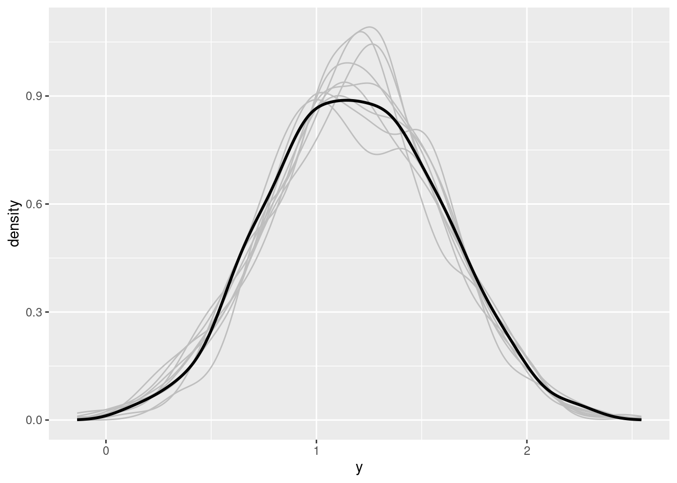
brms::pp_check will produce if applied on a brm object.
Binary Regression Model
rm(list = ls())
library("ggplot2")
library("plyr")
Data Simulation
Data are simulated similarly as for the linear model:
set.seed(123)
N <- 500
df <- data.frame(x_1 = runif(n = N),
                 x_2 = runif(n = N))
(beta_0 <- rnorm(n = 1, mean = 0, sd = .1))
[1] -0.06018928(beta_x_1 <- rnorm(n = 1, mean = 1, sd = .1))[1] 0.9006301(beta_x_2 <- rnorm(n = 1, mean = -.5, sd = .1))[1] -0.3973215df$eta <- beta_0 + beta_x_1 * df$x_1 + beta_x_2 * df$x_2
df$y <- rbinom(n = N, size = 1, prob = plogis(q = df$eta))Visualisations
df$x_1_c <- cut(df$x_1, breaks = seq(0, 1, by = .1),
                include.lowest = T,
                labels = seq(.05, .95, by = .1))
df$x_1_c <- as.numeric(as.character(df$x_1_c))
df_p_A <- ddply(df, c("x_1_c"), summarise,
                p = mean(y > .5))
df_p_A <- data.frame('p' = rep(df_p_A$p, each = 2),
                     'x_1' = sort(c(df_p_A$x_1_c - .05,
                                    df_p_A$x_1_c + .05)))
df_p_B <- data.frame('x_1' = seq(0, 1, by = .01),
                     'p' = plogis(beta_0 +
                                    beta_x_1 * seq(0, 1, by = .01) +
                                    beta_x_2 * .5))
set.seed(0)
ggplot(data = df, aes(x = x_1, y = y)) +
  geom_jitter(aes(color = x_2), width = 0, height = .1) +
  geom_line(data = df_p_A, aes(y = p, group = p)) +
  geom_line(data = df_p_B, aes(y = p), linetype = 2)
## ... 'not as linear as it seems':
# plot(df_p_B$x_1[-1], diff(df_p_B$p))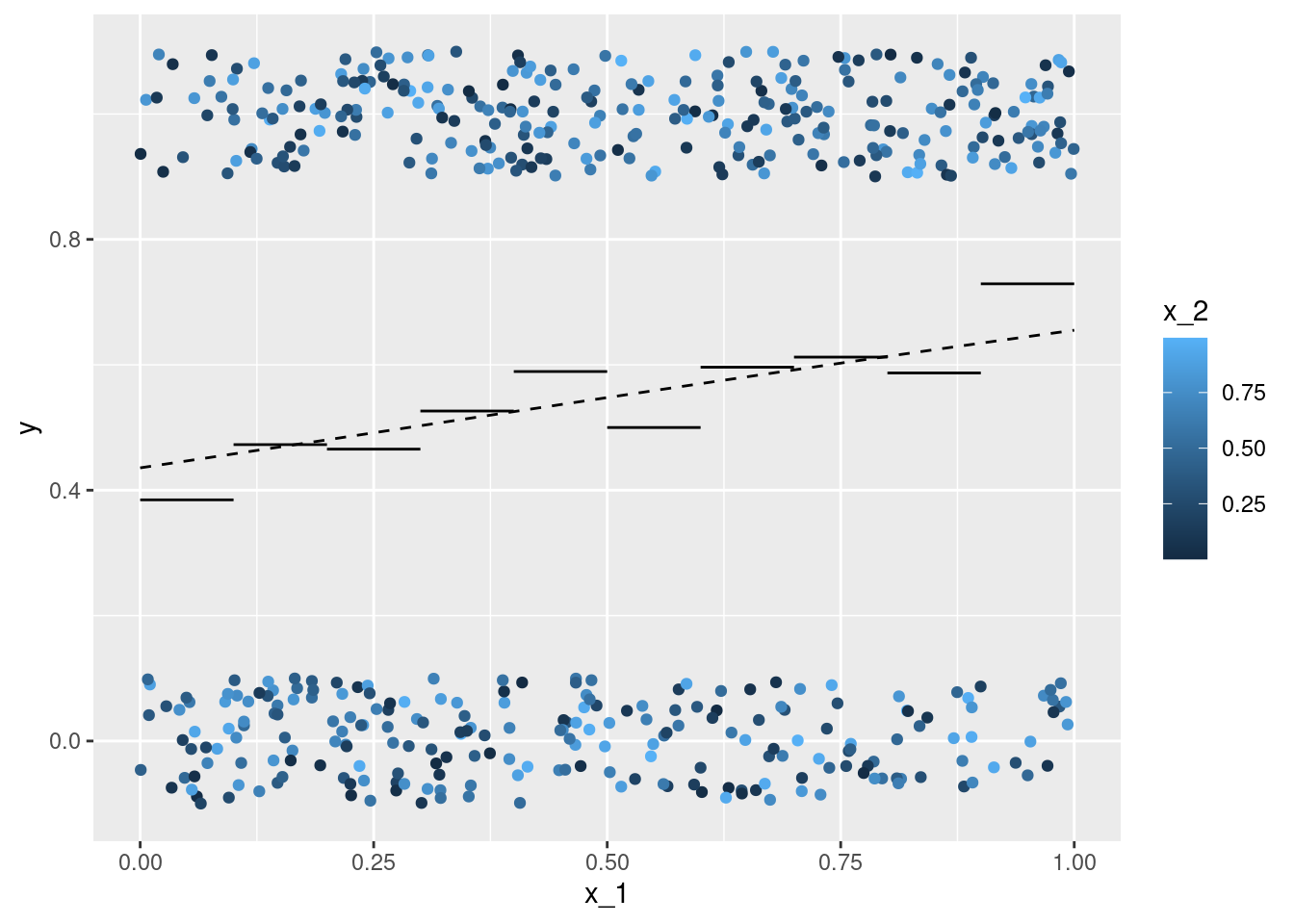
x_1 with response y - each individual observation is coloured according to the second covariate x_2, and additionally ‘jittered’ in vertical direction.
Modeling
The basic R command for (frequentist) estimation of the parameters of a binary regression model is a call to the function glm with family argument binomial:
m <- glm(y ~ x_1 + x_2, data = df,
         family = binomial(link = 'logit'))
summary(m)
Call:
glm(formula = y ~ x_1 + x_2, family = binomial(link = "logit"),
    data = df)

Coefficients:
            Estimate Std. Error z value Pr(>|z|)
(Intercept)  -0.2908     0.2358  -1.233 0.217531
x_1           1.1598     0.3248   3.570 0.000356 ***
x_2          -0.1713     0.3138  -0.546 0.585034
---
Signif. codes:  0 '***' 0.001 '**' 0.01 '*' 0.05 '.' 0.1 ' ' 1

(Dispersion parameter for binomial family taken to be 1)

    Null deviance: 688.53  on 499  degrees of freedom
Residual deviance: 675.30  on 497  degrees of freedom
AIC: 681.3

Number of Fisher Scoring iterations: 4
Visualisations
nd <- data.frame('x_1' = 0:1, 'x_2' = .5)
(nd$eta <- predict(m, newdata = nd, type = 'link'))
1 2
-0.3764387 0.7833343 coef(m)[1] + c(0, 1) * coef(m)[2] + .5 * coef(m)[3][1] -0.3764387 0.7833343pA <- ggplot(data = df, aes(x = x_1, y = eta, color = x_2)) +
geom_point() +
geom_line(data = nd, aes(x = x_1, y = eta, color = x_2))
nd <- data.frame('x_1' = .5,
'x_2' = 0:1)
(nd$eta <- predict(m, newdata = nd, type = 'link')) 1 2
0.2891090 0.1177866 coef(m)[1] + .5 * coef(m)[2] + c(0, 1) * coef(m)[3][1] 0.2891090 0.1177866pB <- ggplot(data = df, aes(x = x_2, y = eta, color = x_1)) +
geom_point() +
geom_line(data = nd, aes(x = x_2, y = eta, color = x_1))
cowplot::plot_grid(pA, pB, ncol = 2)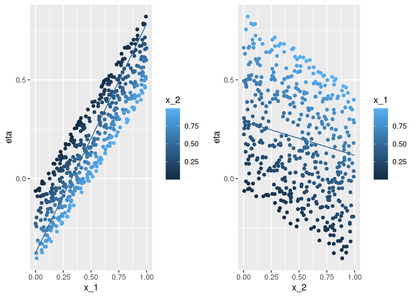
x_1 with the true linear predictor eta - each individual observation is coloured according to the second covariate x_2. The line gives the point estimation for the conditional expectation with the second covariate x_2 fixed to \(0.5\).
nd <- data.frame(x_1 = seq(0, 1, by = .1),
                 x_2 = .5)
(nd$p <- predict(m, newdata = nd, type = 'response'))
[1] 0.4069861 0.4352503 0.4639417 0.4928738 0.5218537 0.5506872 0.5791841
[8] 0.6071630 0.6344556 0.6609111 0.6863983plogis(coef(m)[1] + seq(0, 1, by = .1) * coef(m)[2] +
.5 * coef(m)[3]) [1] 0.4069861 0.4352503 0.4639417 0.4928738 0.5218537 0.5506872 0.5791841
[8] 0.6071630 0.6344556 0.6609111 0.6863983ggplot(data = df, aes(x = x_1, y = y)) +
geom_jitter(aes(color = x_2), width = 0, height = .1) +
geom_line(data = nd, aes(x = x_1, y = p, color = x_2)) +
geom_line(data = df_p_B, aes(y = p), linetype = 2)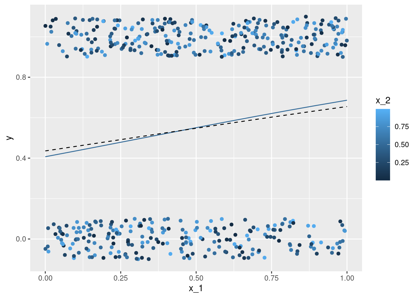
x_1 with the true conditional expectation p - each individual observation is coloured according to the second covariate x_2. The line gives the point estimation for the conditional expectation with the second covariate x_2 fixed to \(0.5\).
Estimated Expected Value
We can apply the Bernstein-von Mises theorem to estimate the expected value:
- Fit the model: Obtain the maximum likelihood estimate for the model’s coefficients (
coef) along with their variance-covariance matrix (vcov). - Simulate coefficients: Perform an ‘informal’ Bayesian posterior simulation using the multivariate normal distribution, based on the Bernstein-von Mises theorem.
- Convert simulated coefficients: Apply an appropriate transformation to the simulated coefficients to compute the simulated quantity of interest. This quantity typically depends on the values of all explanatory variables, and researchers may:
- Focus on a specific observation (usually an ‘average’), or
- Average across all sample observations.
In both cases, the applied transformation incorporates the researcher’s specific choice.
library("MASS")
coef(m)
(Intercept) x_1 x_2
-0.2907775 1.1597730 -0.1713224 vcov(m) (Intercept) x_1 x_2
(Intercept) 0.05560471 -0.048970067 -0.047028038
x_1 -0.04897007 0.105509175 -0.004560743
x_2 -0.04702804 -0.004560743 0.098439583set.seed(0)
B <- mvrnorm(n = 100, mu = coef(m), Sigma = vcov(m))
head(B) (Intercept) x_1 x_2
[1,] -0.08125910 0.6544775 -0.2581602
[2,] -0.40299145 1.3779659 -0.3263178
[3,] 0.09915843 1.0089580 -0.5398310
[4,] 0.03289839 0.8600445 -0.3880109
[5,] -0.12814786 1.3256621 -0.5036957
[6,] -0.55953065 1.4562644 0.3176658nd <- expand.grid('x_1' = nd$x_1,
'x_2' = nd$x_2,
's' = 1:nrow(B))
head(nd) x_1 x_2 s
1 0.0 0.5 1
2 0.1 0.5 1
3 0.2 0.5 1
4 0.3 0.5 1
5 0.4 0.5 1
6 0.5 0.5 1nd$p <- plogis(B[nd$s, 1] + B[nd$s, 2] * nd$x_1 +
B[nd$s, 3] * nd$x_2)
dd <- ddply(nd, c('x_1'), summarise,
p_mean = mean(p),
p_lwr_95 = quantile(p, prob = .025),
p_upr_95 = quantile(p, prob = .975),
p_lwr_9 = quantile(p, prob = .05),
p_upr_9 = quantile(p, prob = .95),
p_lwr_75 = quantile(p, prob = .125),
p_upr_75 = quantile(p, prob = .875))
set.seed(0)
ggplot(data = df, aes(x = x_1)) +
geom_jitter(aes(y = y, color = x_2), width = 0, height = .1) +
geom_ribbon(data = dd, aes(x = x_1, ymin = p_lwr_95,
ymax = p_upr_95), alpha = .4) +
geom_ribbon(data = dd, aes(x = x_1, ymin = p_lwr_9,
ymax = p_upr_9), alpha = .4) +
geom_ribbon(data = dd, aes(x = x_1, ymin = p_lwr_75,
ymax = p_upr_75), alpha = .4) +
geom_line(data = dd, aes(y = p_mean))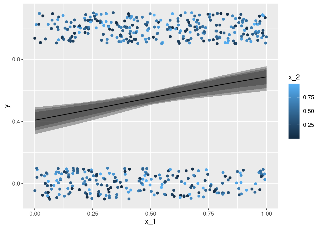
x_1 with the true conditional expectation mu - each individual observation is coloured according to the second covariate x_2. The line gives the point estimation for the conditional expectation with the second covariate x_2 fixed to \(0.5\).
Poisson Regression Model
rm(list = ls())
library("ggplot2")
Data Simulation
Data are simulated similarly as for the linear model:
set.seed(123)
N <- 500
df <- data.frame(x_1 = runif(n = N),
                 x_2 = runif(n = N))
(beta_0 <- rnorm(n = 1, mean = 0, sd = .1))
[1] -0.06018928(beta_x_1 <- rnorm(n = 1, mean = 1, sd = .1))[1] 0.9006301(beta_x_2 <- rnorm(n = 1, mean = -.5, sd = .1))[1] -0.3973215df$eta <- beta_0 + beta_x_1 * df$x_1 + beta_x_2 * df$x_2
df$y <- rpois(n = N, lambda = exp(df$eta))Visualisations
df$x_1_c <- cut(df$x_1, breaks = seq(0, 1, by = .1),
                include.lowest = T,
                labels = seq(.05, .95, by = .1))
df$x_1_c <- as.numeric(as.character(df$x_1_c))
df_p_A <- ddply(df, c("x_1_c"), summarise,
                mu = mean(y))
df_p_A <- data.frame('mu' = rep(df_p_A$mu, each = 2),
                     'x_1' = sort(c(df_p_A$x_1_c - .05,
                                    df_p_A$x_1_c + .05)))
df_p_B <- data.frame('x_1' = seq(0, 1, by = .01),
                     'mu' = exp(beta_0 +
                                  beta_x_1 * seq(0, 1, by = .01) +
                                  beta_x_2 * .5))
set.seed(0)
ggplot(data = df, aes(x = x_1, y = y)) +
  geom_jitter(aes(color = x_2), width = 0, height = .1) +
  geom_line(data = df_p_A, aes(y = mu, group = mu)) +
  geom_line(data = df_p_B, aes(y = mu), linetype = 2)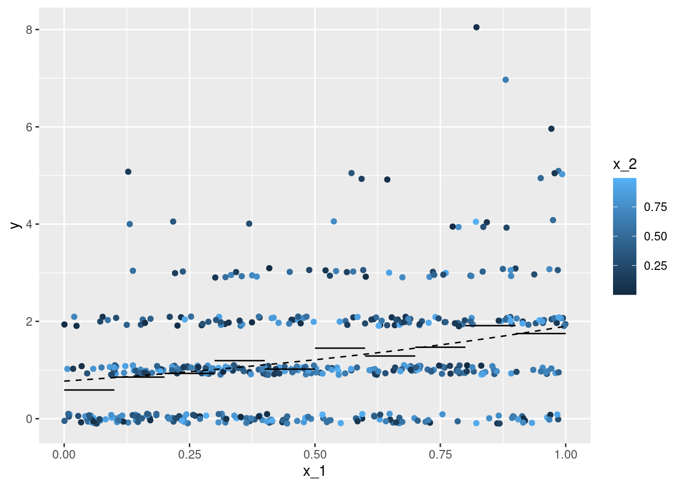
x_1 with response y - each individual observation is coloured according to the second covariate x_2.
Modeling
The basic R command for (frequentist) estimation of the parameters of a binary regression model is a call to the function glm with family argument poisson(link = 'log'):
m <- glm(y ~ x_1 + x_2, data = df, family = poisson(link = 'log'))
summary(m)
Call:
glm(formula = y ~ x_1 + x_2, family = poisson(link = "log"),
    data = df)

Coefficients:
            Estimate Std. Error z value Pr(>|z|)
(Intercept) -0.09637    0.11000  -0.876    0.381
x_1          1.05534    0.14351   7.354 1.93e-13 ***
x_2         -0.54067    0.13875  -3.897 9.74e-05 ***
---
Signif. codes:  0 '***' 0.001 '**' 0.01 '*' 0.05 '.' 0.1 ' ' 1

(Dispersion parameter for poisson family taken to be 1)

    Null deviance: 619.76  on 499  degrees of freedom
Residual deviance: 551.67  on 497  degrees of freedom
AIC: 1395.1

Number of Fisher Scoring iterations: 5
Estimated Expected Value
Let’s again apply the Bernstein-von Mises theorem
library("MASS")
coef(m)
(Intercept) x_1 x_2
-0.09636825 1.05534471 -0.54067416 vcov(m) (Intercept) x_1 x_2
(Intercept) 0.012100215 -0.0115419704 -0.0083283575
x_1 -0.011541970 0.0205956476 -0.0008112633
x_2 -0.008328358 -0.0008112633 0.0192505213set.seed(0)
B <- mvrnorm(n = 100, mu = coef(m), Sigma = vcov(m))
head(B) (Intercept) x_1 x_2
[1,] 0.05743986 0.8596548 -0.5240625
[2,] -0.10120645 1.1692825 -0.5989887
[3,] 0.01910641 0.9263818 -0.7232511
[4,] 0.02386701 0.8912981 -0.6321912
[5,] -0.06117581 1.0833727 -0.7137618
[6,] -0.30539283 1.1687677 -0.3825595nd <- expand.grid('x_1' = seq(0, 1, by = .1),
'x_2' = .5,
's' = 1:nrow(B))
head(nd) x_1 x_2 s
1 0.0 0.5 1
2 0.1 0.5 1
3 0.2 0.5 1
4 0.3 0.5 1
5 0.4 0.5 1
6 0.5 0.5 1nd$mu <- exp(B[nd$s, 1] +
B[nd$s, 2] * nd$x_1 +
B[nd$s, 3] * nd$x_2)
dd <- ddply(nd, c('x_1'), summarise,
mu_mean = mean(mu),
mu_lwr_95 = quantile(mu, prob = .025),
mu_upr_95 = quantile(mu, prob = .975),
mu_lwr_9 = quantile(mu, prob = .05),
mu_upr_9 = quantile(mu, prob = .95),
mu_lwr_75 = quantile(mu, prob = .125),
mu_upr_75 = quantile(mu, prob = .875))
df_p_B <- data.frame('x_1' = seq(0, 1, by = .01),
'mu' = exp(coef(m)[1] +
coef(m)[2] * seq(0, 1, by = .01) +
coef(m)[3] * .5))
set.seed(0)
ggplot(data = df, aes(x = x_1)) +
geom_jitter(aes(y = y, color = x_2), width = 0, height = .1) +
geom_ribbon(data = dd, aes(x = x_1, ymin = mu_lwr_95,
ymax = mu_upr_95), alpha = .4) +
geom_ribbon(data = dd, aes(x = x_1, ymin = mu_lwr_9,
ymax = mu_upr_9), alpha = .4) +
geom_ribbon(data = dd, aes(x = x_1, ymin = mu_lwr_75,
ymax = mu_upr_75), alpha = .4) +
geom_line(data = dd, aes(y = mu_mean)) +
geom_line(data = df_p_B, aes(y = mu), linetype = 2)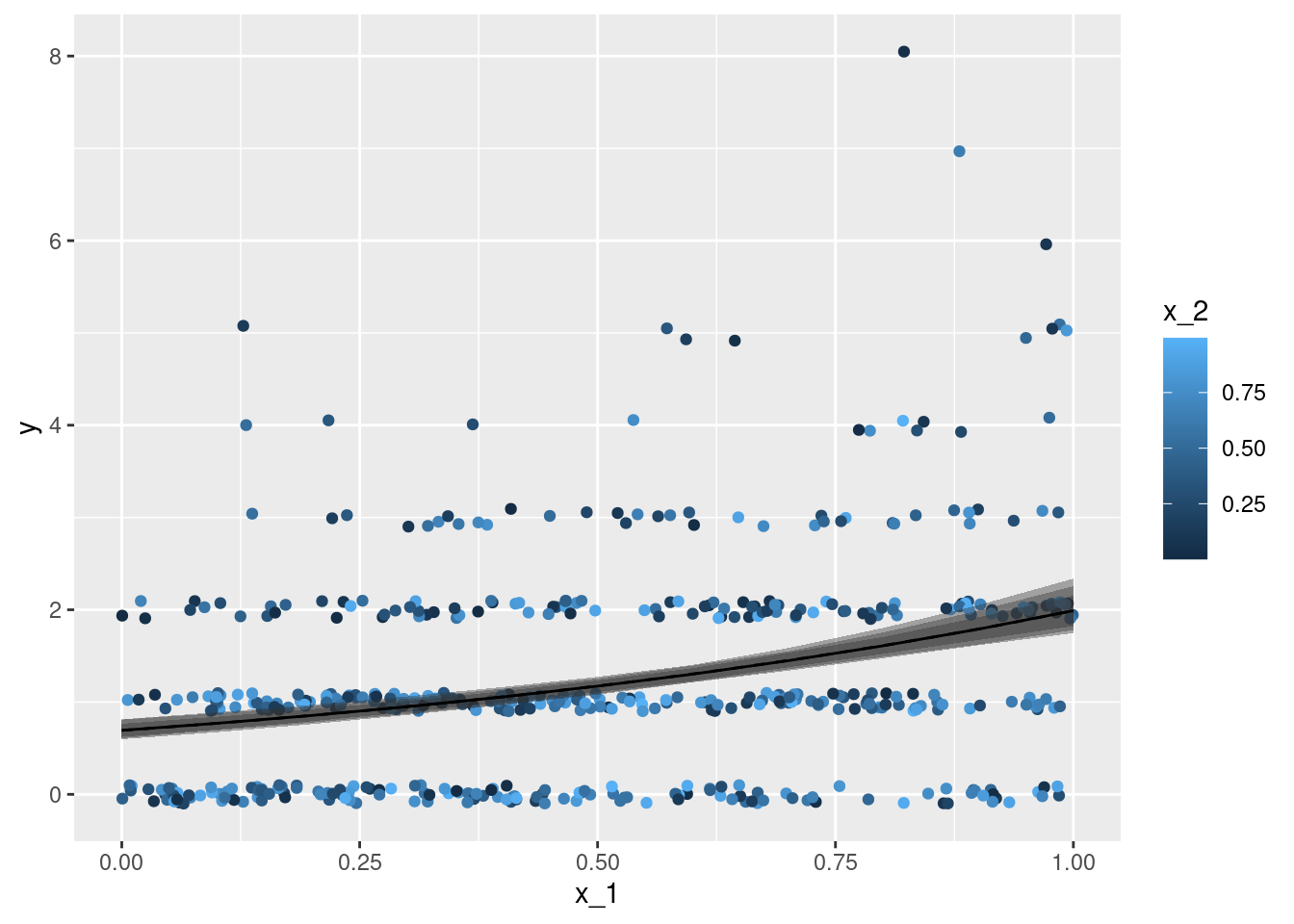
x_1 with the response observations y - each individual observation is coloured according to the second covariate x_2. The line gives the point estimation for the conditional expectation with the second covariate x_2 fixed to \(0.5\), the coloured intervals give point-wise central 75%, 90%, and 95% credible intervals for the conditional expectation.
Mixed models
… a.k.a. hierarchical model, multilevel model, …
rm(list = ls())
library("lme4")
library("ggplot2")
library("plyr")
Data Simulation Function f_sim_data
f_sim_data <- function(seed, type) {
  set.seed(seed) # Set seed for reproducibility
  parameters <- list(## Global intercept:
    "beta_0" = rnorm(n = 1, mean = 2, sd = .1),
    ## Global slope of 'x':
    "beta_x" = rnorm(n = 1, mean = 1.5, sd = .1),
    ## Standard deviation of residuals:
    "sigma" = abs(rnorm(n = 1, mean = 1,
                        sd = .1)))
  if (type == "Random_Intercept") {
    ## Standard deviation of random intercept parameters:
    parameters$'sigma_u' <- abs(rnorm(n = 1, mean = 1, sd = .1))
    ## Number of groups:
    parameters$'G' <- 30
    ## Number of observations per group:
    parameters$'n_per_g' <- 30
    g <- rep(1:parameters$'G', each = parameters$'n_per_g')
    x <- runif(n = parameters$'G' * parameters$'n_per_g',
               min = -1, max = 1)
    df <- data.frame('x' = x,
                     'g' = g)
    df$u <- rnorm(n = parameters$'G', mean = 0,
                  sd = parameters$'sigma_u')[df$g]
    df$mu <- parameters$'beta_0' +
      parameters$'beta_x' * df$x + df$u
    attributes(df)$'type' <- type
    attributes(df)$'parameters' <- parameters
  }
  if (type == "Nested") {
    ## Standard deviation of random intercept parameters:
    parameters$'sigma_u_a' <- abs(rnorm(n = 1, mean = 1, sd = .1))
    parameters$'sigma_u_b' <- abs(rnorm(n = 1, mean = 1, sd = .1))
    ## Number of groups in 1st level:
    parameters$'G_a' <- 30
    ## Number of observations per group:
    parameters$'n_per_g_a' <- 30
    ## Number of groups in 2nd level:
    parameters$'G_b' <- 10
    ## Number of observations per group:
    parameters$'n_per_g_b' <- 6
    gr <- as.data.frame(expand.grid('g_a' = 1:parameters$'G_a',
                                    'g_b' = 1:parameters$'G_b'))
    df <- gr[rep(1:nrow(gr), each = parameters$'n_per_g_b'), ]
    df <- df[order(df$g_a, df$g_b), ]
    rownames(df) <- NULL
    df$g_ab <- paste0(df$g_a, "_", df$g_b)
    df$x <- runif(n = parameters$'G_a' * parameters$'n_per_g_a',
                  min = -1, max = 1)
    u_a <- rnorm(n = parameters$'G_a', mean = 0,
                 sd = parameters$'sigma_u_a')
    df$u_a <- u_a[df$g_a]
    u_b <- rnorm(n = length(unique(df$g_ab)), mean = 0,
                 sd = parameters$'sigma_u_b')
    names(u_b) <- unique(df$g_ab)
    df$u_b <- as.numeric(u_b[df$g_ab])
    df$mu <- parameters$'beta_0' + parameters$'beta_x' * df$x +
      df$u_a + df$u_b
    attributes(df)$'type' <- type
    attributes(df)$'parameters' <- parameters
  }
  epsilon <- rnorm(n = nrow(df), mean = 0, sd = parameters$'sigma')
  df$y <- df$mu + epsilon
  return(df)
}
Random Intercept Model
df <- f_sim_data(seed = 0, type = "Random_Intercept")
head(df)
x g u mu y
1 0.3215956 1 -1.095936 1.50226149 2.9095988
2 0.2582281 1 -1.095936 1.40927751 2.1118975
3 -0.8764275 1 -1.095936 -0.25568956 -0.1425014
4 -0.5880509 1 -1.095936 0.16746754 2.2155593
5 -0.6468865 1 -1.095936 0.08113349 -1.6210895
6 0.3740457 1 -1.095936 1.57922556 1.9028505unlist(attributes(df)$parameters) beta_0 beta_x sigma sigma_u G n_per_g
2.126295 1.467377 1.132980 1.127243 30.000000 30.000000 m <- lmer(y ~ x + (1 | g), data = df)
summary(m)Linear mixed model fit by REML ['lmerMod']
Formula: y ~ x + (1 | g)
Data: df
REML criterion at convergence: 2889.6
Scaled residuals:
Min 1Q Median 3Q Max
-3.10483 -0.67888 -0.01549 0.67941 2.97945
Random effects:
Groups Name Variance Std.Dev.
g (Intercept) 1.421 1.192
Residual 1.287 1.134
Number of obs: 900, groups: g, 30
Fixed effects:
Estimate Std. Error t value
(Intercept) 2.00545 0.22090 9.078
x 1.51171 0.06674 22.652
Correlation of Fixed Effects:
(Intr)
x 0.000 … small simulation study
R <- 50
ci_df <- NULL
for (r in 1:R) {
  ## Simulate data:
  df <- f_sim_data(seed = r, type = "Random_Intercept")
  ## Estimate models:
  lm_model <- lm(y ~ x, data = df)
  lmer_model <- lmer(y ~ x + (1 | g), data = df)
  ## Extract confidence intervals:
  lm_ci <- confint(lm_model, level = 0.95)
  lmer_ci <- suppressMessages(confint(lmer_model, level = 0.95))
  ## Store results:
  par_name <- "sigma"
  tmp <- data.frame(r = r,
                    par_name = par_name,
                    Value = rep(attributes(df)$parameters$sigma,
                                times = 2),
                    Model = c("lm", "lmer"),
                    Estimate = c(summary(lm_model)$sigma,
                                 summary(lmer_model)$sigma),
                    CI_Low = rep(NA, 2),
                    CI_High = c(NA, 2))
  ci_df <- rbind(ci_df, tmp)
  par_name <- "x"
  tmp <- data.frame(r = r,
                    par_name = par_name,
                    Value = rep(attributes(df)$parameters$beta_x,
                                times = 2),
                    Model = c("lm", "lmer"),
                    Estimate = c(coef(lm_model)[par_name],
                                 fixef(lmer_model)[par_name]),
                    CI_Low = c(lm_ci[par_name, 1],
                               lmer_ci[par_name, 1]),
                    CI_High = c(lm_ci[par_name, 2],
                                lmer_ci[par_name, 2]))
  ci_df <- rbind(ci_df, tmp)
  par_name <- "(Intercept)"
  tmp <- data.frame(r = r,
                    par_name = par_name,
                    Value = rep(attributes(df)$parameters$beta_0,
                                times = 2),
                    Model = c("lm", "lmer"),
                    Estimate = c(coef(lm_model)[par_name],
                                 fixef(lmer_model)[par_name]),
                    CI_Low = c(lm_ci[par_name, 1],
                               lmer_ci[par_name, 1]),
                    CI_High = c(lm_ci[par_name, 2],
                                lmer_ci[par_name, 2]))
  ci_df <- rbind(ci_df, tmp)
  cat(".")
}
ci_df$par_name <- factor(ci_df$par_name,
levels = c("(Intercept)", "x", "sigma"))ggplot(ci_df, aes(x = r)) +
geom_pointrange(aes(y = Estimate, ymin = CI_Low,
ymax = CI_High)) +
geom_point(aes(y = Value), color = 2) +
labs(y = "Parameter estimate & interval",
x = "Simulation run") +
facet_grid(cols = vars(Model), rows = vars(par_name),
scales = "free") +
theme(legend.position = "none")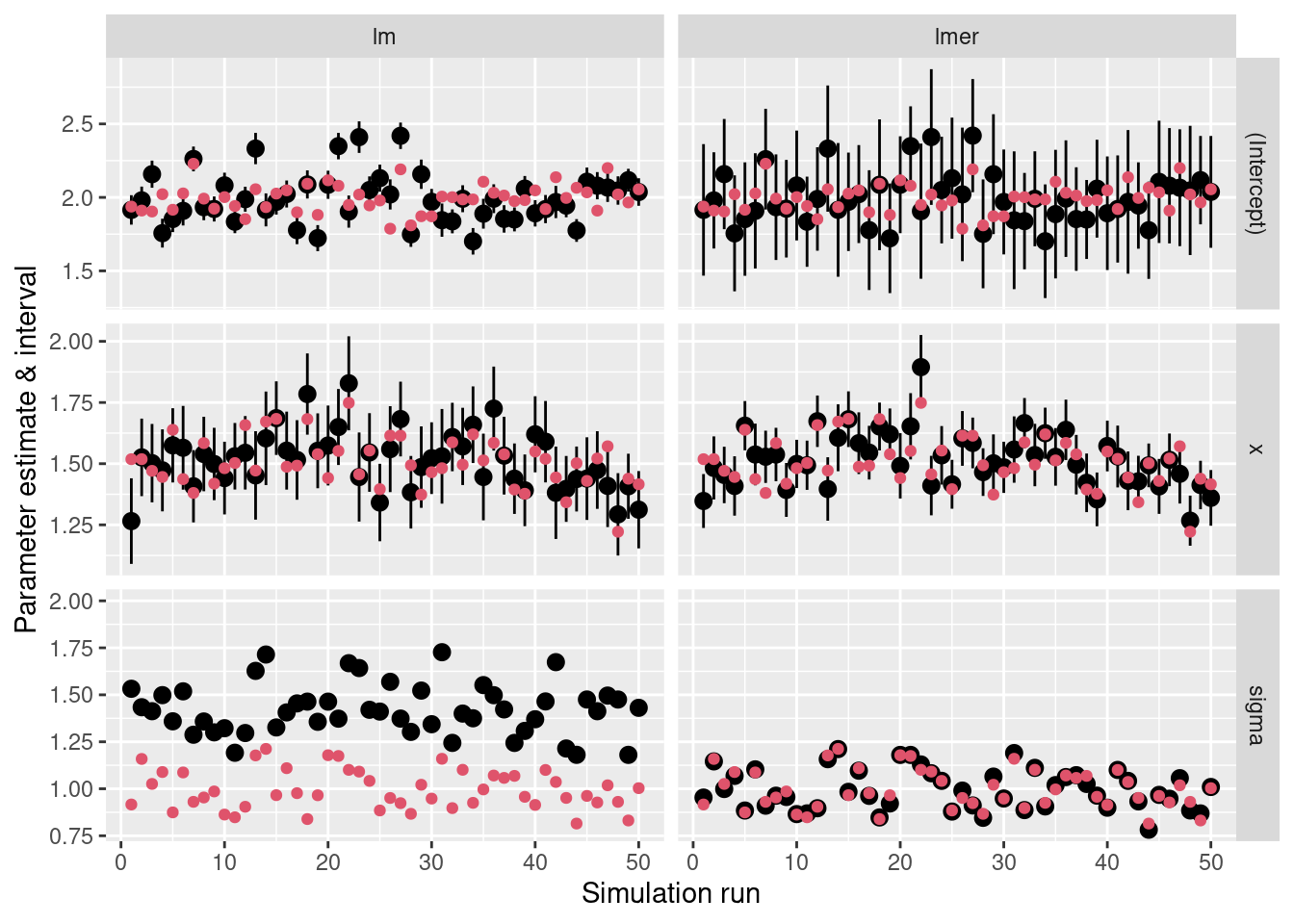
Random Intercept with Random Slope Model
f_add_random_slope <- function(df, x_lab, g_lab) {
  ## assign(paste0("sigma_u_", x_label, "_", g_label), 1)
  sigma_u_slope <- abs(rnorm(n = 1, mean = 1, sd = .1))
  u_slope <- rnorm(length(unique(df[, g_lab])), mean = 0,
                   sd = sigma_u_slope)
  df$u_slope <- u_slope[df[, g_lab]]
  df$y <- df$y + df[, x_lab] * df$u_slope
  attributes(df)$parameters[[paste0("sigma_u_", x_lab, "_", g_lab)]] <-
    sigma_u_slope
  return(df)
}
df <- f_sim_data(seed = 0, type = "Random_Intercept")
df <- f_add_random_slope(df = df, x_lab = "x", g_lab = "g")
head(df)
x g u mu y u_slope
1 0.3215956 1 -1.095936 1.50226149 2.4603313 -1.396995
2 0.2582281 1 -1.095936 1.40927751 1.7511541 -1.396995
3 -0.8764275 1 -1.095936 -0.25568956 1.0818636 -1.396995
4 -0.5880509 1 -1.095936 0.16746754 3.0370635 -1.396995
5 -0.6468865 1 -1.095936 0.08113349 -0.7173922 -1.396995
6 0.3740457 1 -1.095936 1.57922556 1.3803104 -1.396995gr <- expand.grid('x' = c(-1, 1),
'g' = 1:attributes(df)$parameters$G)
dd <- ddply(df, c("g"), summarise,
'intercept' = u[1],
'slope' = u_slope[1])
gr$y <- attributes(df)$parameters$beta_0 + dd$intercept[gr$g] +
gr$x * (attributes(df)$parameters$beta_x + dd$slope[gr$g])
ggplot(data = df, aes(x = x, y = y)) +
geom_line(data = data.frame(x = c(-1, 1),
y = attributes(df)$parameters$beta_0 +
c(-1, 1) *
attributes(df)$parameters$beta_x)) +
geom_point(alpha = .5) +
geom_line(data = gr, aes(group = g), linetype = 2) +
facet_wrap(~ g)
unlist(attributes(df)$parameters) beta_0 beta_x sigma sigma_u G n_per_g
2.126295 1.467377 1.132980 1.127243 30.000000 30.000000
sigma_u_x_g
1.066731 m <- lmer(y ~ x + (1 + x|g), data = df)
summary(m)Linear mixed model fit by REML ['lmerMod']
Formula: y ~ x + (1 + x | g)
Data: df
REML criterion at convergence: 2969.4
Scaled residuals:
Min 1Q Median 3Q Max
-2.73036 -0.66985 -0.01614 0.65063 2.87938
Random effects:
Groups Name Variance Std.Dev. Corr
g (Intercept) 1.410 1.187
x 1.488 1.220 0.03
Residual 1.299 1.140
Number of obs: 900, groups: g, 30
Fixed effects:
Estimate Std. Error t value
(Intercept) 2.0000 0.2202 9.084
x 1.3435 0.2328 5.772
Correlation of Fixed Effects:
(Intr)
x 0.024 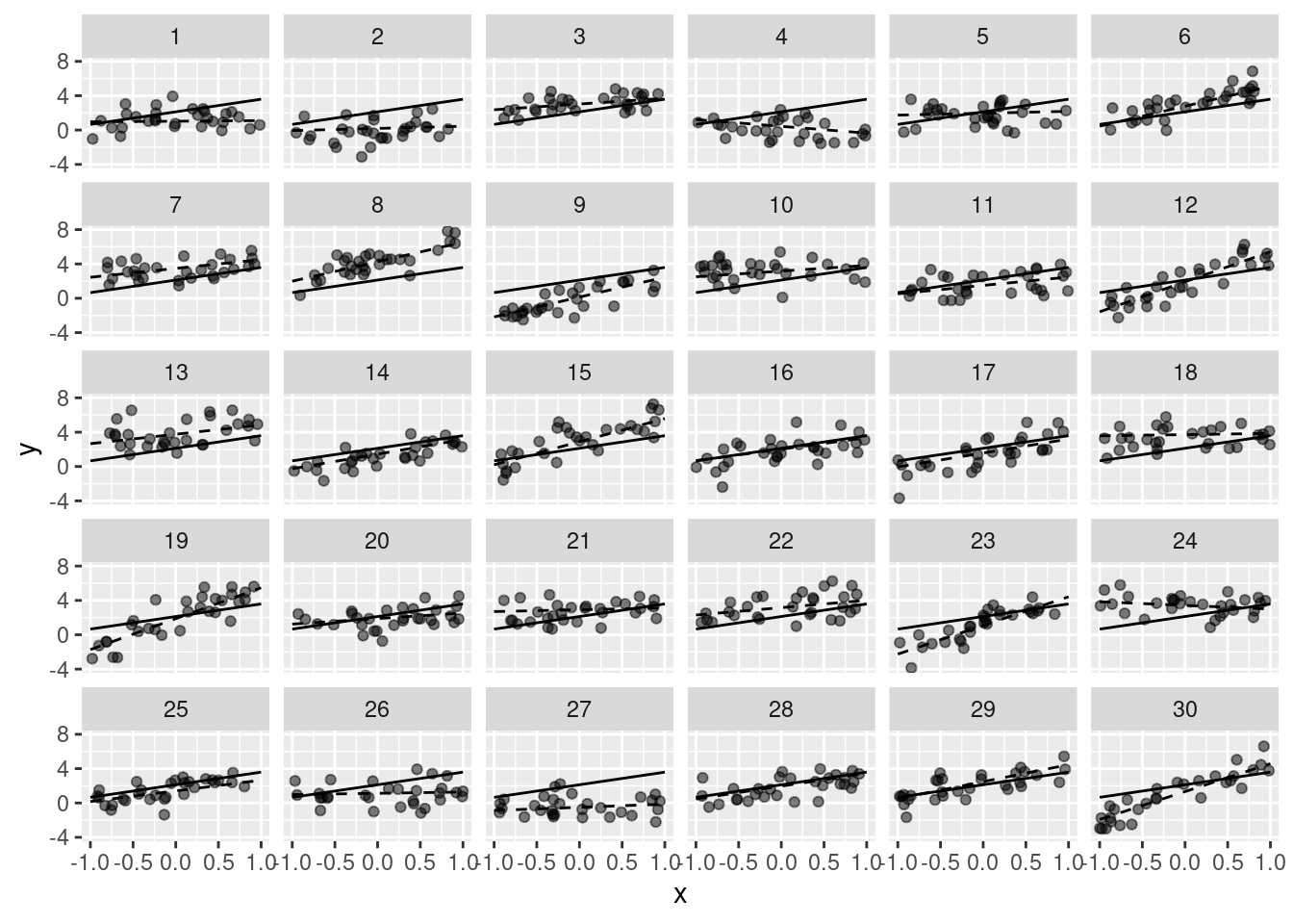
Nested Model
df <- f_sim_data(seed = 0, type = "Nested")
head(df)
g_a g_b g_ab x u_a u_b mu y
1 1 1 1_1 -0.8764275 -1.936757 0.6458663 -0.45064437 -0.8523900
2 1 1 1_1 -0.5880509 -1.936757 0.6458663 -0.02748727 0.1857836
3 1 1 1_1 -0.6468865 -1.936757 0.6458663 -0.11382132 0.9328256
4 1 1 1_1 0.3740457 -1.936757 0.6458663 1.38427075 3.8232376
5 1 1 1_1 -0.2317926 -1.936757 0.6458663 0.49527783 -0.7620346
6 1 1 1_1 0.5396828 -1.936757 0.6458663 1.62732283 2.7937350## ... two alternatives:
m1 <- lmer(y ~ x + (1|g_a/g_b), data = df)
m2 <- lmer(y ~ x + (1|g_a) + (1|g_ab), data = df)
unlist(attributes(df)$parameters) beta_0 beta_x sigma sigma_u_a sigma_u_b G_a n_per_g_a G_b
2.126295 1.467377 1.132980 1.127243 1.041464 30.000000 30.000000 10.000000
n_per_g_b
6.000000 summary(m1)Linear mixed model fit by REML ['lmerMod']
Formula: y ~ x + (1 | g_a/g_b)
Data: df
REML criterion at convergence: 6235.4
Scaled residuals:
Min 1Q Median 3Q Max
-3.06066 -0.65621 0.02234 0.63566 2.79567
Random effects:
Groups Name Variance Std.Dev.
g_b:g_a (Intercept) 0.8489 0.9214
g_a (Intercept) 1.4214 1.1922
Residual 1.3809 1.1751
Number of obs: 1800, groups: g_b:g_a, 300; g_a, 30
Fixed effects:
Estimate Std. Error t value
(Intercept) 2.10415 0.22578 9.319
x 1.41589 0.05253 26.954
Correlation of Fixed Effects:
(Intr)
x 0.001 summary(m2)Linear mixed model fit by REML ['lmerMod']
Formula: y ~ x + (1 | g_a) + (1 | g_ab)
Data: df
REML criterion at convergence: 6235.4
Scaled residuals:
Min 1Q Median 3Q Max
-3.06066 -0.65621 0.02234 0.63566 2.79567
Random effects:
Groups Name Variance Std.Dev.
g_ab (Intercept) 0.8489 0.9214
g_a (Intercept) 1.4214 1.1922
Residual 1.3809 1.1751
Number of obs: 1800, groups: g_ab, 300; g_a, 30
Fixed effects:
Estimate Std. Error t value
(Intercept) 2.10415 0.22578 9.319
x 1.41589 0.05253 26.954
Correlation of Fixed Effects:
(Intr)
x 0.001 cowplot::plot_grid(
ggplot(data = data.frame(x = ranef(m1)$'g_a'[, 1],
y = ranef(m2)$'g_a'[, 1])) +
geom_point(aes(x = x, y = y)) +
geom_abline(intercept = 0, slope = 1) +
labs(x = "ranef(m1)$'g_a'[, 1]", y = "ranef(m2)$'g_a'[, 1]"),
ggplot(data = data.frame(x = sort(ranef(m1)$'g_b:g_a'[, 1]),
y = sort(ranef(m2)$'g_ab'[, 1]))) +
geom_point(aes(x = x, y = y)) +
geom_abline(intercept = 0, slope = 1) +
labs(x = "sort(ranef(m1)$'g_b:g_a'[, 1])",
y = "sort(ranef(m2)$'g_ab'[, 1])"))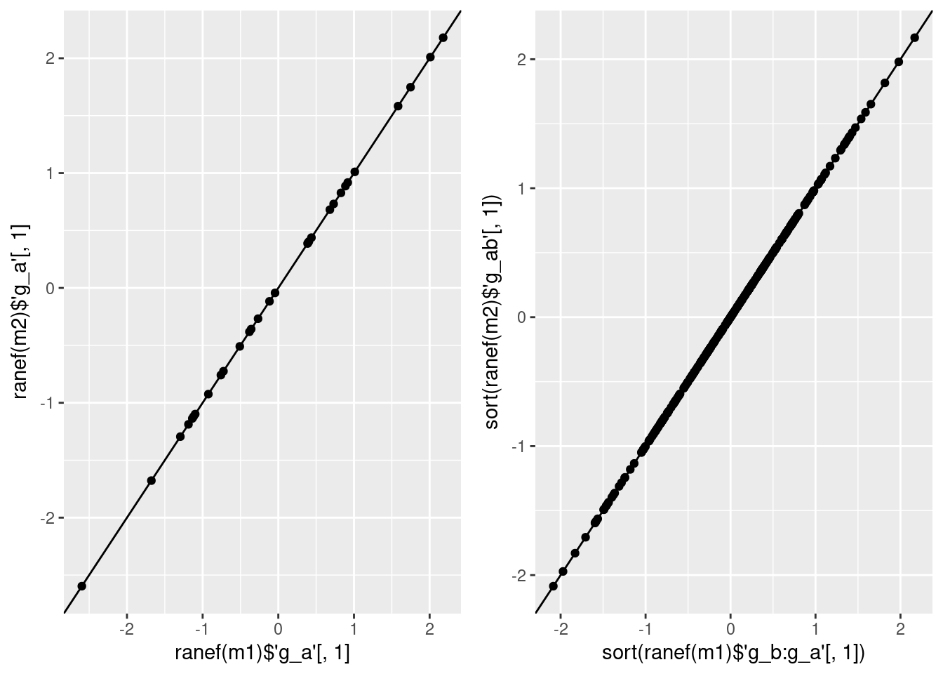
… add covariate ‘z’ as constant within 2nd level
f_add_covariate_constant_within_b <- function(df) {
  attributes(df)$'parameters'$'beta_z' <- rnorm(n = 1, mean = 1.5,
                                                sd = .1)
  if (attributes(df)$type != "Nested") {
    stop("Use type 'Nested' to generate 'df'.")
  }
  z <- runif(n = length(unique(df$g_ab)), min = -1, max = 1)
  names(z) <- unique(df$g_ab)
  df$z <- as.numeric(z[df$g_ab])
  df$y <- df$y + df$z * attributes(df)$'parameters'$'beta_z'
  return(df)
}
df <- f_sim_data(seed = 0, type = "Nested")
df <- f_add_covariate_constant_within_b(df = df)
ggplot(data = df, aes(x = x, y = y, colour = z)) +
  geom_point() +
  facet_wrap(~ g_a) +
  theme(legend.position = 'top')
m <- lmer(y ~ x + z + (1 | g_a / g_b), data = df)
summary(m)
Linear mixed model fit by REML ['lmerMod']
Formula: y ~ x + z + (1 | g_a/g_b)
Data: df
REML criterion at convergence: 6236.8
Scaled residuals:
Min 1Q Median 3Q Max
-3.05900 -0.66108 0.02254 0.63115 2.78727
Random effects:
Groups Name Variance Std.Dev.
g_b:g_a (Intercept) 0.848 0.9209
g_a (Intercept) 1.429 1.1955
Residual 1.381 1.1751
Number of obs: 1800, groups: g_b:g_a, 300; g_a, 30
Fixed effects:
Estimate Std. Error t value
(Intercept) 2.09644 0.22647 9.257
x 1.41538 0.05253 26.943
z 1.72034 0.11487 14.976
Correlation of Fixed Effects:
(Intr) x
x 0.001
z -0.033 -0.009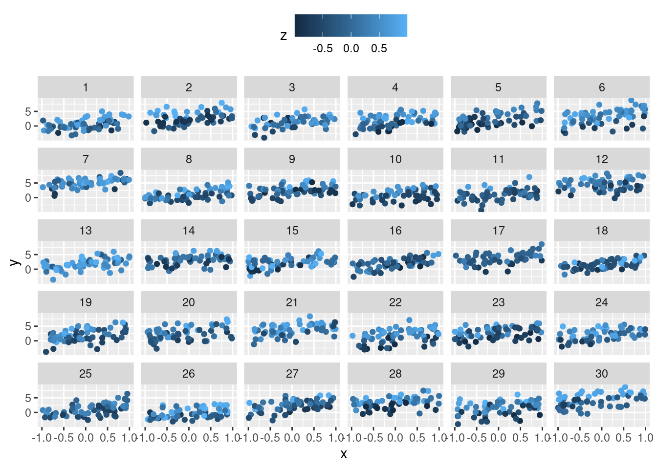
Flexible Models
… a.k.a. GAMs …
rm(list = ls())
library("mgcv")library("ggplot2")
library("plyr")
library("colorspace")A ‘simple’ GAM
… to see what’s going on ‘under the hood’ …
We begin with simulating data by using an underlying effect function for the single covariate x which is rather non-linear:
n <- 100
set.seed(123)
df <- data.frame(x = runif(n, min = 0, max = pi))
df$y <- sin(df$x^2 - pi) + rnorm(n, sd = .25)
nd <- data.frame(x = seq(0, pi, length.out = 50))
nd$mu <- sin(nd$x^2 - pi)
ggplot(data = df, aes(x = x)) +
  geom_point(aes(y = y)) +
  geom_line(data = nd, aes(y = mu), linetype = "dashed")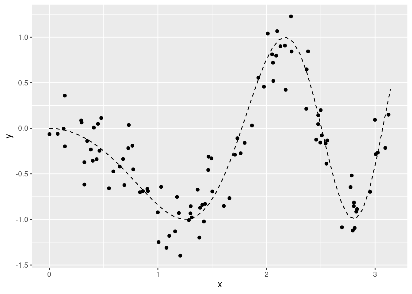
A suitable model can be implemented using the function mgcv::gam, with in especially usage of the function mgcv:s():
m <- gam(y ~ s(x), data = df)
plot(m)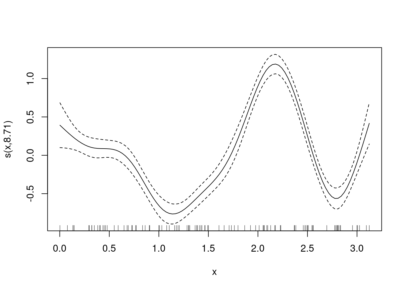
nd$pre <- predict(m, newdata = nd)
ggplot(data = df, aes(x = x)) +
  geom_point(aes(y = y)) +
  geom_line(data = nd, aes(y = mu), linetype = "dashed") +
  geom_line(data = nd, aes(y = pre))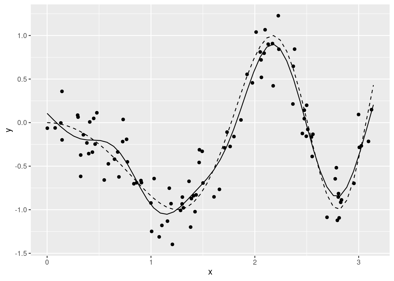
What does s() do?
X <- predict(m, newdata = nd, type = "lpmatrix")
head(X)
(Intercept) s(x).1 s(x).2 s(x).3 s(x).4 s(x).5 s(x).6
1 1 -1.110390 -0.7863538 1.327113 -1.0156741 -1.389606 -0.5755292
2 1 -1.112745 -0.7620022 1.330739 -0.9857403 -1.394499 -0.5443745
3 1 -1.114827 -0.7374878 1.332975 -0.9534962 -1.395550 -0.5091587
4 1 -1.116216 -0.7124827 1.331685 -0.9156141 -1.387345 -0.4648478
5 1 -1.116234 -0.6862777 1.323491 -0.8674136 -1.362650 -0.4065304
6 1 -1.114115 -0.6580194 1.304598 -0.8038132 -1.313750 -0.3295964
s(x).7 s(x).8 s(x).9
1 -1.841987 -0.6428615 -1.758172
2 -1.836490 -0.5718634 -1.686202
3 -1.820364 -0.5005500 -1.614233
4 -1.780468 -0.4285334 -1.542263
5 -1.704336 -0.3554311 -1.470294
6 -1.580454 -0.2808812 -1.398324Xd <- reshape2::melt(X)
head(Xd) Var1 Var2 value
1 1 (Intercept) 1
2 2 (Intercept) 1
3 3 (Intercept) 1
4 4 (Intercept) 1
5 5 (Intercept) 1
6 6 (Intercept) 1Xd$x <- nd$x[Xd$Var1]
ggplot(data = Xd, aes(x = x, y = value, group = Var2, color = Var2)) +
geom_line() +
scale_color_discrete_qualitative(pal = "Dark2") +
labs(color = "Basis function:")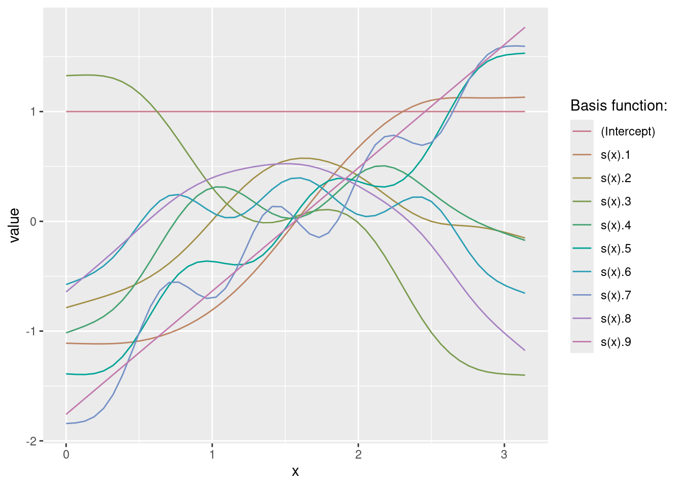
(b <- coef(m))(Intercept) s(x).1 s(x).2 s(x).3 s(x).4 s(x).5
-0.2883327 0.1328587 3.3990351 2.6033203 3.3949996 -1.9450739
s(x).6 s(x).7 s(x).8 s(x).9
2.6219341 -0.1327275 -6.4627018 1.3564139 nd$eta_hat <- as.numeric(b %*% t(X))
ggplot(data = df, aes(x = x)) +
geom_line(data = nd, aes(y = pre)) +
geom_line(data = nd, aes(y = eta_hat), color = 2, linetype = "dotted", size = 5)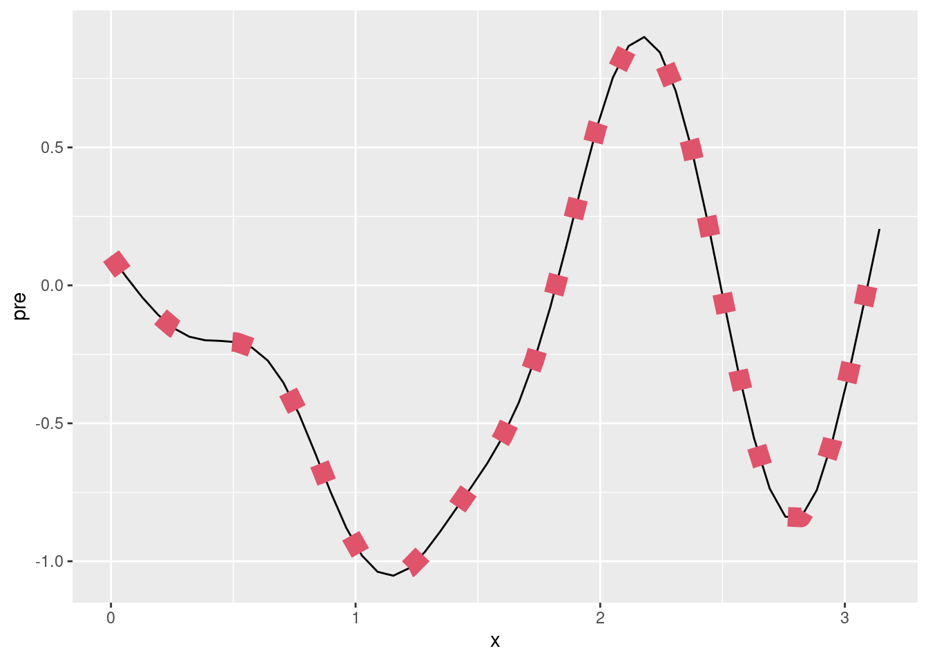
How does mgcv quantify uncertainty and how can we interpret this uncertainty?
B <- rmvn(50, coef(m), vcov(m))
head(B)
(Intercept) s(x).1 s(x).2 s(x).3 s(x).4 s(x).5 s(x).6
[1,] -0.2969723 0.14827346 2.845380 2.472228 2.986735 -2.025393 2.321902
[2,] -0.2798226 0.45813882 2.791453 2.539675 2.988796 -1.225334 1.925825
[3,] -0.2989047 0.02970708 3.627493 2.644463 3.434373 -1.716172 2.719180
[4,] -0.2998487 -0.16155372 4.105077 2.831955 3.863112 -2.421325 3.100904
[5,] -0.3156754 0.32549077 3.244017 2.692452 3.153326 -1.978761 2.526919
[6,] -0.2895788 0.11326272 1.954769 2.364647 2.358708 -1.651279 1.594067
s(x).7 s(x).8 s(x).9
[1,] -0.10699650 -5.629549 1.6480470
[2,] -0.15590646 -5.349300 0.8544413
[3,] -0.32639388 -6.690499 1.3949870
[4,] -0.30574994 -7.587330 1.9507888
[5,] 0.07690747 -6.235893 1.2065182
[6,] -0.05222090 -4.137128 1.8122858E <- t(X %*% t(B))
Ed <- reshape2::melt(E)
head(Ed) Var1 Var2 value
1 1 1 -0.05497982
2 2 1 0.16933401
3 3 1 0.10640081
4 4 1 0.07715345
5 5 1 0.18366364
6 6 1 -0.26333221Ed$x <- nd$x[Ed$Var2]
ggplot(data = Ed, aes(x = x, y = value, group = Var1)) +
geom_line(alpha = .3)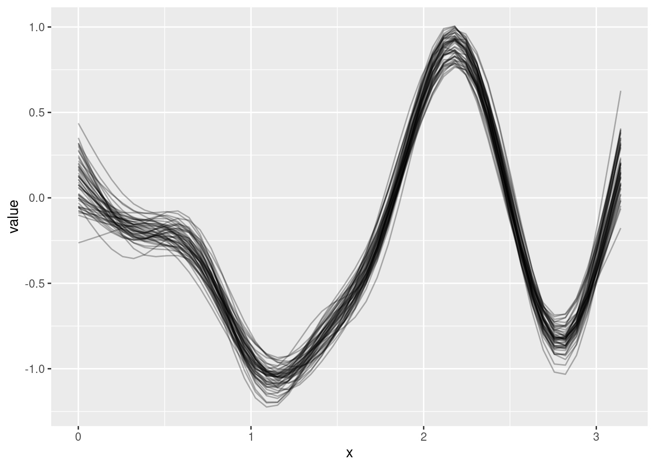
B <- rmvn(1000, coef(m), vcov(m))
E <- t(X %*% t(B))
Ed <- reshape2::melt(E)
Ed$x <- nd$x[Ed$Var2]
mean(fitted(m))
[1] -0.2883327dd <- ddply(Ed, c("x"), summarise,
m = mean(value),
lwr = quantile(value, prob = .025),
upr = quantile(value, prob = .975))
plot(m)
lines(dd$x, dd$lwr - mean(fitted(m)), col = 2)
lines(dd$x, dd$upr - mean(fitted(m)), col = 2)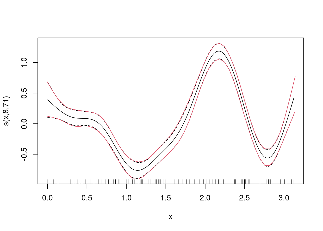
GAM with bivariate effect surface
Let’s see how a ‘spatial’ effect is estimated?
n <- 500
set.seed(123)
df <- data.frame(x1 = runif(n, min = 0, max = pi),
                 x2 = runif(n, min = 0, max = pi))
df$y <- sin(df$x1 * df$x2 - pi) + rnorm(n, sd = .25)
nd <- expand.grid('x1' = seq(0, pi, length.out = 50),
                  'x2' = seq(0, pi, length.out = 50))
nd$mu <- sin(nd$x1 * nd$x2 - pi)
ggplot(data = nd, aes(x = x1, y = x2)) +
  geom_contour_filled(aes(z = mu)) +
  geom_point(data = df) +
  scale_fill_discrete_divergingx(pal = "Zissou")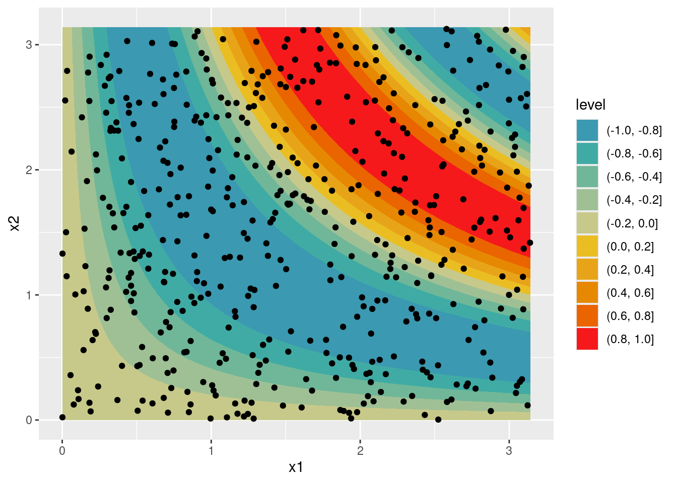
m_s <- gam(y ~ s(x1, x2), data = df)
m_t2 <- gam(y ~ t2(x1, x2), data = df)
# plot(m, scheme = 3)
# plot(m, scheme = 3)
nd_all <- data.frame(x1 = rep(nd$x1, 3),
                     x2 = rep(nd$x2, 3),
                     value = c(nd$mu,
                               predict(m_s, newdata = nd),
                               predict(m_t2, newdata = nd)),
                     type = factor(rep(c("mu", "gam(y ~ s(x1, x2), ...)",
                                  "gam(y ~ t2(x1, x2), ...)"), each = nrow(nd)),
                                  levels = c("mu", "gam(y ~ s(x1, x2), ...)",
                                  "gam(y ~ t2(x1, x2), ...)")))
ggplot(data = nd_all, aes(x = x1, y = x2)) +
  geom_contour_filled(aes(z = value)) +
  facet_wrap(~ type) +
  theme(legend.position = "top") +
  labs(fill = "Value:") +
  scale_fill_discrete_divergingx(pal = "Zissou")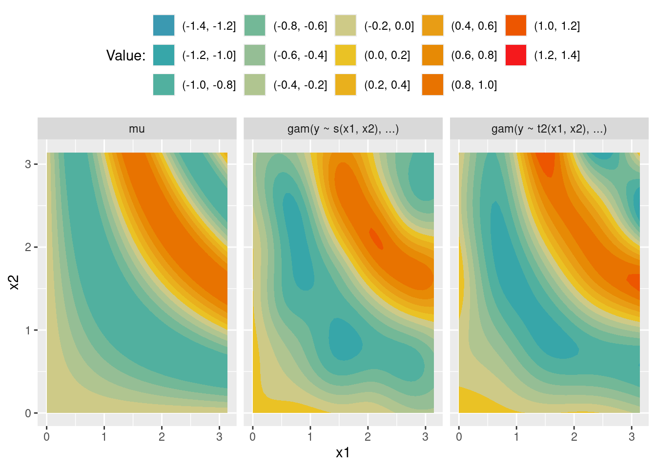
X <- predict(m_s, newdata = nd, type = "lpmatrix")
head(X)
(Intercept) s(x1,x2).1 s(x1,x2).2 s(x1,x2).3 s(x1,x2).4 s(x1,x2).5
1 1 1.976689 0.03371151 0.3304568 -0.00259226 0.17111069
2 1 1.953387 0.12968114 0.3370067 0.03879382 0.10776499
3 1 1.924786 0.22810439 0.3459613 0.08379769 0.03947457
4 1 1.890669 0.32877303 0.3576584 0.13285743 -0.03302845
5 1 1.850898 0.43139923 0.3722188 0.18626423 -0.10880938
6 1 1.805536 0.53566289 0.3894894 0.24424418 -0.18664853
s(x1,x2).6 s(x1,x2).7 s(x1,x2).8 s(x1,x2).9 s(x1,x2).10 s(x1,x2).11
1 -0.5733509 0.8731026 -2.546673 0.08897994 -0.4737068 0.09007722
2 -0.5875089 0.9045996 -2.406345 0.20978069 -0.4791941 0.15745018
3 -0.6019473 0.9322257 -2.247393 0.34624806 -0.4797606 0.24512764
4 -0.6168661 0.9548019 -2.071011 0.49751798 -0.4743269 0.35294021
5 -0.6322095 0.9713239 -1.879590 0.66173468 -0.4617458 0.47919667
6 -0.6478180 0.9808658 -1.677758 0.83608598 -0.4410087 0.61933769
s(x1,x2).12 s(x1,x2).13 s(x1,x2).14 s(x1,x2).15 s(x1,x2).16 s(x1,x2).17
1 -0.133159173 0.3158998 0.57525679 -0.1031087 0.5078509 2.222795
2 -0.064956212 0.3701460 0.48745809 -0.2523885 0.4790495 2.247128
3 -0.009115991 0.4244009 0.38551631 -0.4190865 0.4564703 2.258474
4 0.033048128 0.4778276 0.26922983 -0.5988628 0.4397291 2.253921
5 0.060832282 0.5293748 0.13932143 -0.7855388 0.4280232 2.231165
6 0.075409006 0.5777002 -0.00269943 -0.9703603 0.4190936 2.189777
s(x1,x2).18 s(x1,x2).19 s(x1,x2).20 s(x1,x2).21 s(x1,x2).22 s(x1,x2).23
1 -0.18884460 -0.6125473 1.09973055 1.8396779 -0.0333665 -0.9116247
2 -0.16806566 -0.6704053 0.91084502 1.6182853 -0.2572698 -0.9223023
3 -0.14436797 -0.7255835 0.69258252 1.3446765 -0.5065067 -0.9603384
4 -0.11731578 -0.7754304 0.44852400 1.0302451 -0.7734789 -1.0253060
5 -0.08652054 -0.8171072 0.18547182 0.6908278 -1.0478943 -1.1150764
6 -0.05265184 -0.8476338 -0.08790494 0.3518045 -1.3176351 -1.2227076
s(x1,x2).24 s(x1,x2).25 s(x1,x2).26 s(x1,x2).27 s(x1,x2).28 s(x1,x2).29
1 -0.22749543 -0.3291015 0.24309550 -1.116626 -1.743114 -1.7187
2 -0.18306547 -0.3293340 0.13345644 -1.112899 -1.671289 -1.7187
3 -0.13372568 -0.3219909 -0.01411312 -1.110753 -1.599464 -1.7187
4 -0.07912184 -0.3039526 -0.19647388 -1.108954 -1.527639 -1.7187
5 -0.01949693 -0.2731051 -0.40588347 -1.106313 -1.455814 -1.7187
6 0.04461223 -0.2291873 -0.63085090 -1.101163 -1.383989 -1.7187Xd <- reshape2::melt(X)
head(Xd) Var1 Var2 value
1 1 (Intercept) 1
2 2 (Intercept) 1
3 3 (Intercept) 1
4 4 (Intercept) 1
5 5 (Intercept) 1
6 6 (Intercept) 1Xd$x1 <- nd$x1[Xd$Var1]
Xd$x2 <- nd$x2[Xd$Var1]
ggplot(data = Xd, aes(x = x1, y = x2)) +
geom_contour_filled(aes(z = value)) +
facet_wrap(~ Var2) +
theme(legend.position = "top") +
labs(fill = "Value:") +
scale_fill_discrete_divergingx(pal = "Zissou")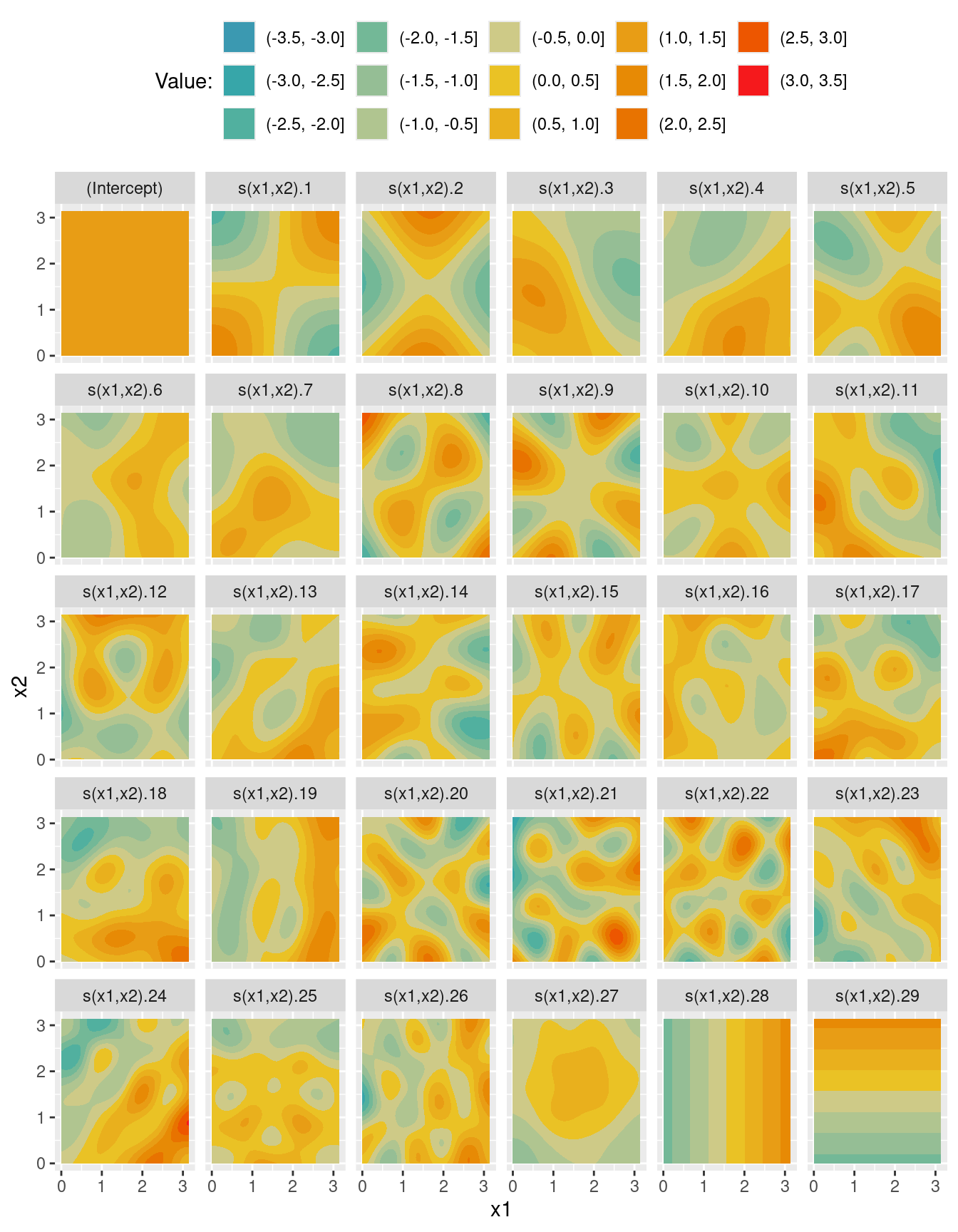
X <- predict(m_t2, newdata = nd, type = "lpmatrix")
Xd <- reshape2::melt(X)
Xd$x1 <- nd$x1[Xd$Var1]
Xd$x2 <- nd$x2[Xd$Var1]
ggplot(data = Xd, aes(x = x1, y = x2)) +
  geom_contour_filled(aes(z = value)) +
  facet_wrap(~ Var2) +
  theme(legend.position = "top") +
  labs(fill = "Value:") +
  scale_fill_discrete_divergingx(pal = "Zissou")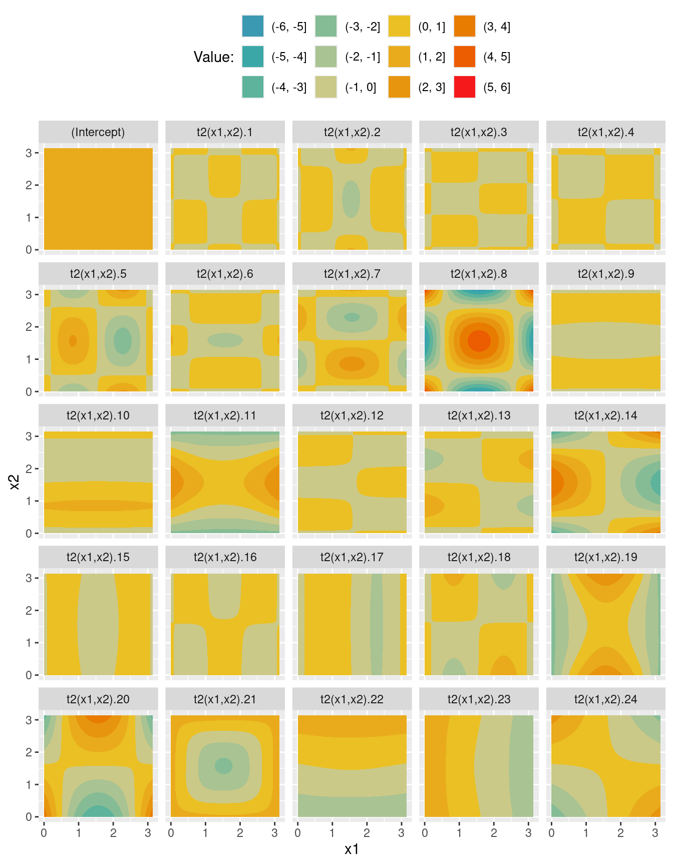
Meet the ocat family …
In order to specifiy an orderled logistic regression in mgcv, we need to specify the family attribute as ocat:
rm(list = ls())
get_prob <- function(lp, theta) {
  R <- length(theta)
  prob <- matrix(0, length(lp), R + 2)
  prob[, R + 2] <- 1
  for (i in 1:R) {
    x <- theta[i] - lp
    ind <- x > 0
    prob[ind, i + 1] <- 1/(1 + exp(-x[ind]))
    ex <- exp(x[!ind])
    prob[!ind, i + 1] <- ex/(1 + ex)
  }
  prob <- t(diff(t(prob)))
  return(prob)
}
get_y <- function(alpha, eta) {
  R <- length(alpha) - 1
  n <- length(eta)
  y <- rep(NA, n)
  u <- eta + qlogis(runif(n)) ## df$mu + log(u/(1-u))
  for (i in 1:R) {
    y[(u > alpha[i]) & (u <= alpha[i + 1])] <- i
  }
  return(y)
}
set.seed(123)
n <- 1000
x <- runif(n, min = -2, max = 2)
df <- data.frame(x = x,
                 eta = x)
alpha <- c(-Inf, -1, 1, 3, Inf)
df$y <- get_y(alpha, df$eta)
df$xc <- cut(df$x, breaks = seq(-2, 2, by = .25), include.lowest = T)
ggplot(data = df, aes(x = xc, y = y)) +
  geom_count(aes(color = after_stat(n)), size = 10) +
  scale_color_continuous_divergingx(pal = "Zissou", mid = 25)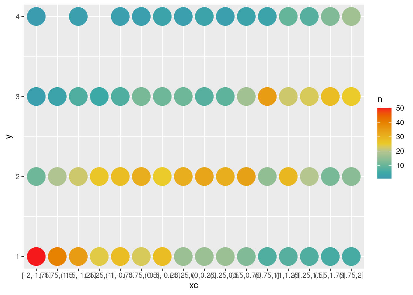
(tmp <- addmargins(xtabs(~ y + xc, data = df), mar = 1)) xc
y [-2,-1.75] (-1.75,-1.5] (-1.5,-1.25] (-1.25,-1] (-1,-0.75] (-0.75,-0.5]
1 50 40 35 24 28 23
2 11 19 22 26 28 31
3 2 3 7 5 7 12
4 1 0 2 0 2 2
Sum 64 62 66 55 65 68
xc
y (-0.5,-0.25] (-0.25,0] (0,0.25] (0.25,0.5] (0.5,0.75] (0.75,1] (1,1.25]
1 28 16 16 16 13 7 8
2 25 31 33 31 34 15 29
3 11 11 8 9 17 35 22
4 3 2 3 2 3 3 10
Sum 67 60 60 58 67 60 69
xc
y (1.25,1.5] (1.5,1.75] (1.75,2]
1 7 6 6
2 20 12 14
3 23 28 25
4 8 13 17
Sum 58 59 62tmp <- tmp[1:4, ] / tmp[5, ]
dfp <- data.frame(y = as.ordered(rep(as.numeric(rownames(tmp)), ncol(tmp))),
x = rep(seq(-1.875, 1.875, by = .25), each = nrow(tmp)),
p = as.numeric(tmp))
ggplot(data = dfp, aes(x = x, y = p, group = y, color = y)) +
geom_point() +
scale_color_discrete_diverging() +
ylim(c(0, 1)) + xlim(c(-2, 2))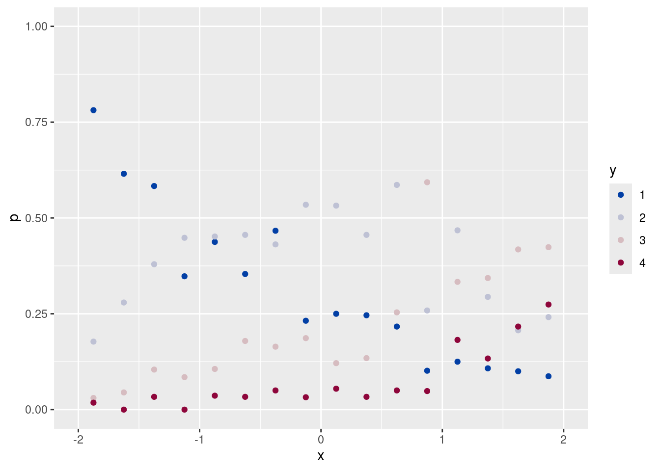
m <- gam(y ~ x, family = ocat(R = 4), data = df)
m$family$getTheta(TRUE)
[1] -1.000000 1.016038 2.978357nd <- data.frame(x = seq(-2, 2, by = .25))
pre <- NULL
pre_here <- predict(m, newdata = nd, type = "response")
head(pre_here) [,1] [,2] [,3] [,4]
1 0.7185518 0.2318687 0.04230184 0.007277626
2 0.6683642 0.2696485 0.05278585 0.009201425
3 0.6140344 0.3087177 0.06562008 0.011627813
4 0.5567073 0.3474112 0.08119694 0.014684548
5 0.4978290 0.3837381 0.09990317 0.018529778
6 0.4390108 0.4155539 0.12207729 0.023358032pre_here <- as.data.frame(pre_here)
pre_here$x <- nd$x
pre_here <- data.frame(x = rep(pre_here$x),
y = rep(1:4, each = nrow(pre_here)),
pre = c(pre_here$V1, pre_here$V2,
pre_here$V3, pre_here$V4))
pre <- rbind(pre, pre_here)
ggplot(data = dfp, aes(x = x, y = p)) +
geom_point(aes(color = y)) +
geom_line(data = pre, aes(x = x, y = pre, group = y, color = factor(y))) +
scale_color_discrete_diverging() +
ylim(c(0, 1)) + xlim(c(-2, 2))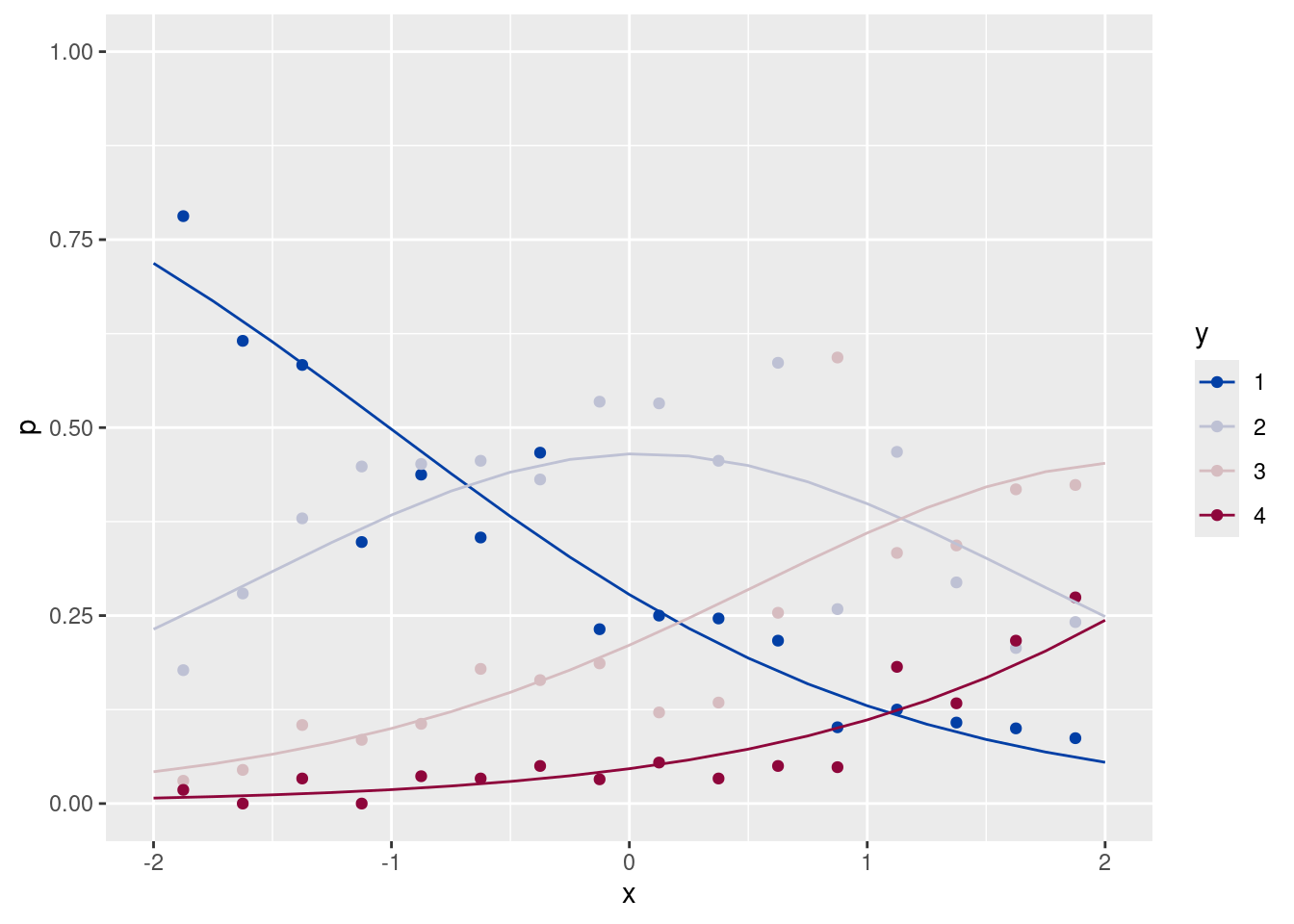
X <- predict(m, newdata = nd, type = "lpmatrix")
## simulate directly from Gaussian approximate posterior...
B <- rmvn(1000, coef(m), vcov(m))
head(B)
(Intercept) x
[1,] -0.105028632 0.8930572
[2,] -0.046419889 0.9389411
[3,] -0.198145365 1.0089490
[4,] -0.030374057 1.0747553
[5,] -0.004272592 0.9200827
[6,] 0.122328585 1.0898455## Alternatively use MH sampling...
# B <- gam.mh(m,thin=2,ns=2000,rw.scale=.15)
E <- t(X %*% t(B))
dim(E)[1] 1000 17theta <- m$family$getTheta(TRUE)
Ps <- apply(X = E, MARGIN = 1, FUN = get_prob,
theta = m$family$getTheta(TRUE))
dim(Ps)[1] 68 1000Pa <- array(dim = c(nrow(nd), 4, nrow(Ps)), data = Ps)
Pa[, , 1] [,1] [,2] [,3] [,4]
[1,] 0.70912598 0.2390743 0.04418099 0.007618715
[2,] 0.66102799 0.2750429 0.05442265 0.009506425
[3,] 0.60935799 0.3119790 0.06680675 0.011856272
[4,] 0.55511268 0.3484444 0.08166458 0.014778299
[5,] 0.49952145 0.3827506 0.09932088 0.018407057
[6,] 0.44394205 0.4130906 0.12006121 0.022906127
[7,] 0.38973107 0.4377095 0.14408647 0.028472967
[8,] 0.33811470 0.4550866 0.17145492 0.035343769
[9,] 0.29008498 0.4641016 0.20201561 0.043797817
[10,] 0.24633870 0.4641590 0.23534177 0.054160495
[11,] 0.20726350 0.4552551 0.27067766 0.066803717
[12,] 0.17296407 0.4379780 0.30691584 0.082142052
[13,] 0.14331460 0.4134422 0.34262085 0.100622384
[14,] 0.11802234 0.3831640 0.37610903 0.122704596
[15,] 0.09668989 0.3488968 0.40558240 0.148830948
[16,] 0.07886846 0.3124477 0.42930113 0.179382695
[17,] 0.06409872 0.2755080 0.44576865 0.214624646nd_all <- NULL
for (k in 1:4) {
tmp <- data.frame(x = nd$x,
y = k,
p_mean = apply(X = Pa, MAR = c(1, 2), FUN = mean)[, k],
p_lwr = apply(X = Pa, MAR = c(1, 2), FUN = quantile, prob = .025)[, k],
p_upr = apply(X = Pa, MAR = c(1, 2), FUN = quantile, prob = .975)[, k])
nd_all <- rbind(nd_all, tmp)
}
ggplot(data = nd_all, aes(x = x, color = y, group = y)) +
geom_ribbon(aes(ymin = p_lwr, ymax = p_upr, fill = y), alpha = .2, color = NA) +
geom_line(aes(y = p_mean)) +
ylim(c(0, 1)) + xlim(c(-2, 2))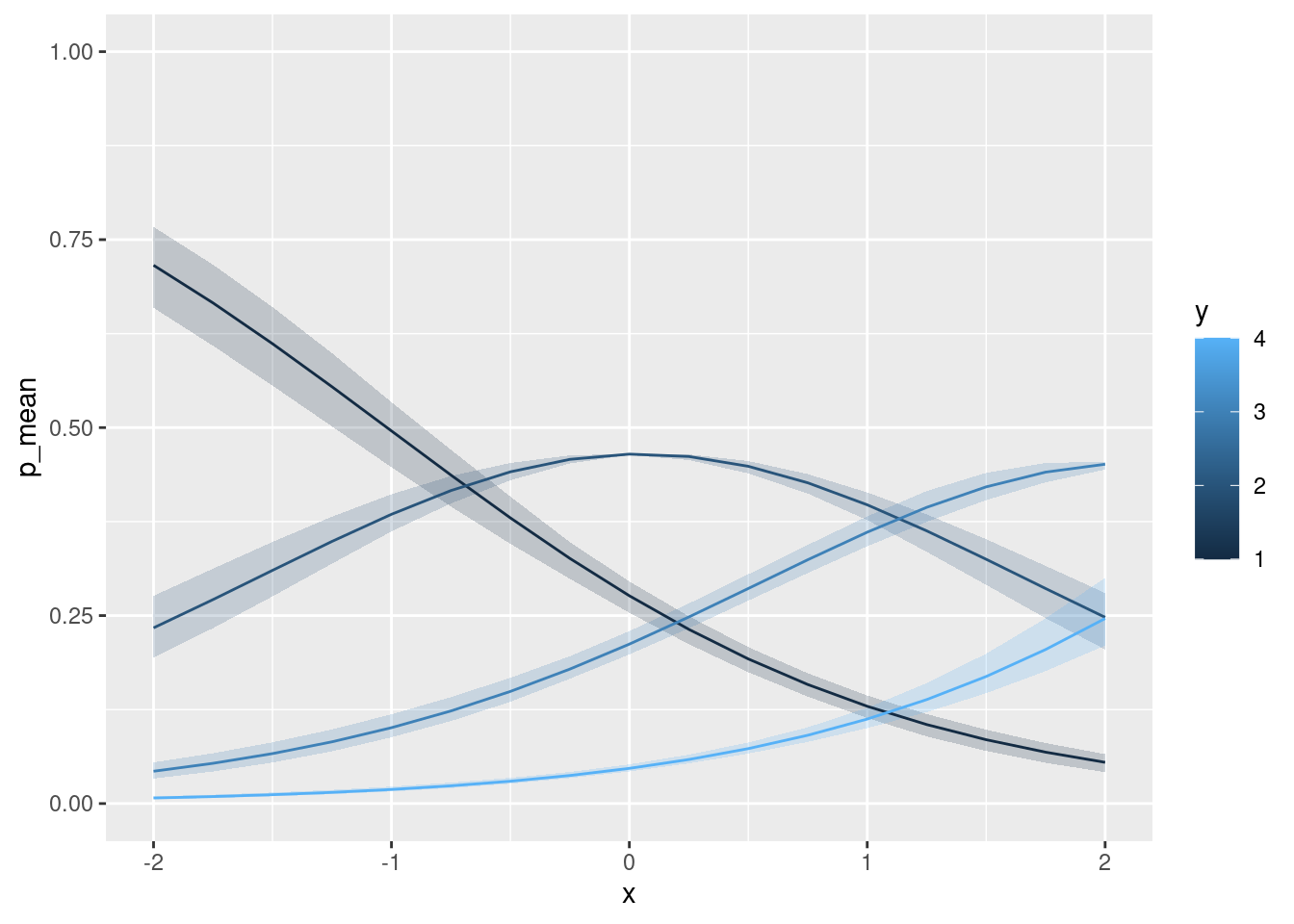
… add a ‘smooth’ …
m <- gam(y ~ s(x), family = ocat(R = 4), data = df)
plot(m)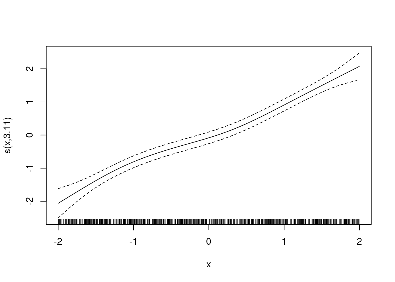
m$family$getTheta(TRUE)[1] -1.000000 1.015276 2.997751nd <- data.frame(x = seq(-2, 2, by = .25))
pre <- NULL
pre_here <- predict(m, newdata = nd, type = "response")
head(pre_here) [,1] [,2] [,3] [,4]
1 0.7528150 0.2052566 0.03593709 0.005991324
2 0.6828033 0.2588899 0.04985119 0.008455591
3 0.6057981 0.3143940 0.06800380 0.011804091
4 0.5306624 0.3638872 0.08947424 0.015976125
5 0.4655438 0.4017491 0.11206784 0.020639208
6 0.4126987 0.4278687 0.13397439 0.025458164pre_here <- as.data.frame(pre_here)
pre_here$x <- nd$x
pre_here <- data.frame(x = rep(pre_here$x),
y = rep(1:4, each = nrow(pre_here)),
pre = c(pre_here$V1, pre_here$V2,
pre_here$V3, pre_here$V4))
pre <- rbind(pre, pre_here)
ggplot(data = dfp, aes(x = x, y = p)) +
geom_point(aes(color = y)) +
geom_line(data = pre, aes(x = x, y = pre, group = y, color = factor(y))) +
scale_color_discrete_diverging() +
ylim(c(0, 1)) + xlim(c(-2, 2))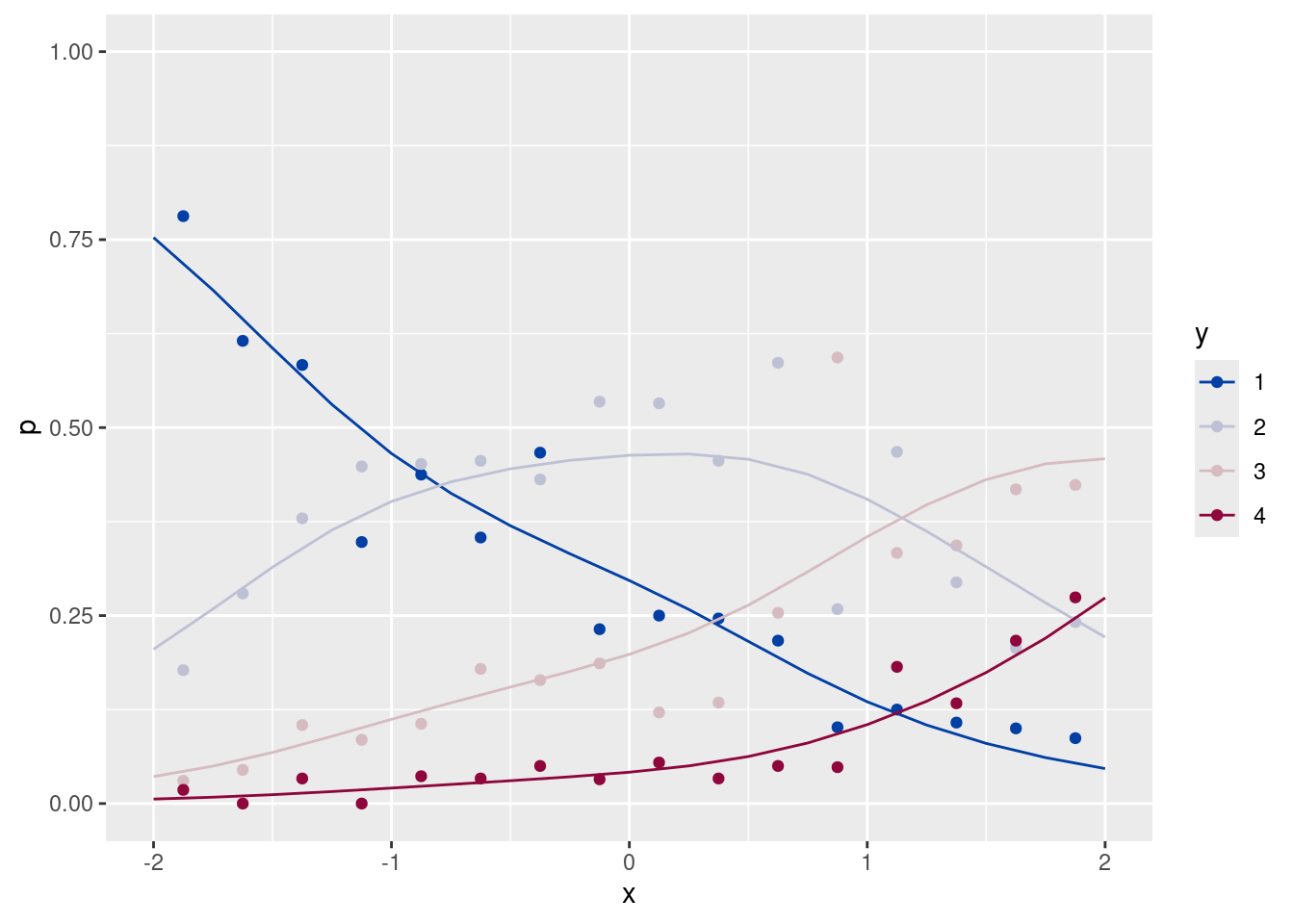
X <- predict(m, newdata = nd, type = "lpmatrix")
## simulate directly from Gaussian approximate posterior...
#B <- rmvn(1000, coef(m), vcov(m))
#head(B)
## Alternatively use MH sampling...
B <- gam.mh(m, thin = 2,ns=2000,rw.scale=.15)$bsE <- t(X %*% t(B))
theta <- m$family$getTheta(TRUE)
Ps <- apply(X = E, MARGIN = 1, FUN = get_prob,
            theta = m$family$getTheta(TRUE))
dim(Ps)
[1] 68 1000Pa <- array(dim = c(nrow(nd), 4, nrow(Ps)), data = Ps)
Pa[, , 1] [,1] [,2] [,3] [,4]
[1,] 0.75047723 0.2070884 0.03636801 0.006066369
[2,] 0.65301954 0.2808443 0.05647650 0.009659665
[3,] 0.55385477 0.3491910 0.08238272 0.014571499
[4,] 0.47461187 0.3968153 0.10865680 0.019916072
[5,] 0.41787029 0.4255307 0.13166394 0.024935069
[6,] 0.37742610 0.4423437 0.15083999 0.029390192
[7,] 0.34812836 0.4521444 0.16649619 0.033231056
[8,] 0.32106312 0.4590603 0.18250871 0.037367850
[9,] 0.28404220 0.4644860 0.20724768 0.044224139
[10,] 0.23356921 0.4621532 0.24746382 0.056813764
[11,] 0.18044007 0.4424674 0.30013219 0.076960322
[12,] 0.13832609 0.4080436 0.35101412 0.102616177
[13,] 0.11098421 0.3726589 0.38816306 0.128193799
[14,] 0.09265203 0.3411394 0.41383132 0.152377306
[15,] 0.07525918 0.3038575 0.43683783 0.184045515
[16,] 0.05628693 0.2528658 0.45550573 0.235341571
[17,] 0.03977246 0.1973141 0.45582264 0.307090775nd_all <- NULL
for (k in 1:4) {
tmp <- data.frame(x = nd$x,
y = k,
p_mean = apply(X = Pa, MAR = c(1, 2), FUN = mean)[, k],
p_lwr = apply(X = Pa, MAR = c(1, 2), FUN = quantile,
prob = .025)[, k],
p_upr = apply(X = Pa, MAR = c(1, 2), FUN = quantile,
prob = .975)[, k])
nd_all <- rbind(nd_all, tmp)
}
ggplot(data = nd_all, aes(x = x, color = y, group = y)) +
geom_ribbon(aes(ymin = p_lwr, ymax = p_upr, fill = y), alpha = .2, color = NA) +
geom_line(aes(y = p_mean)) +
ylim(c(0, 1)) + xlim(c(-2, 2))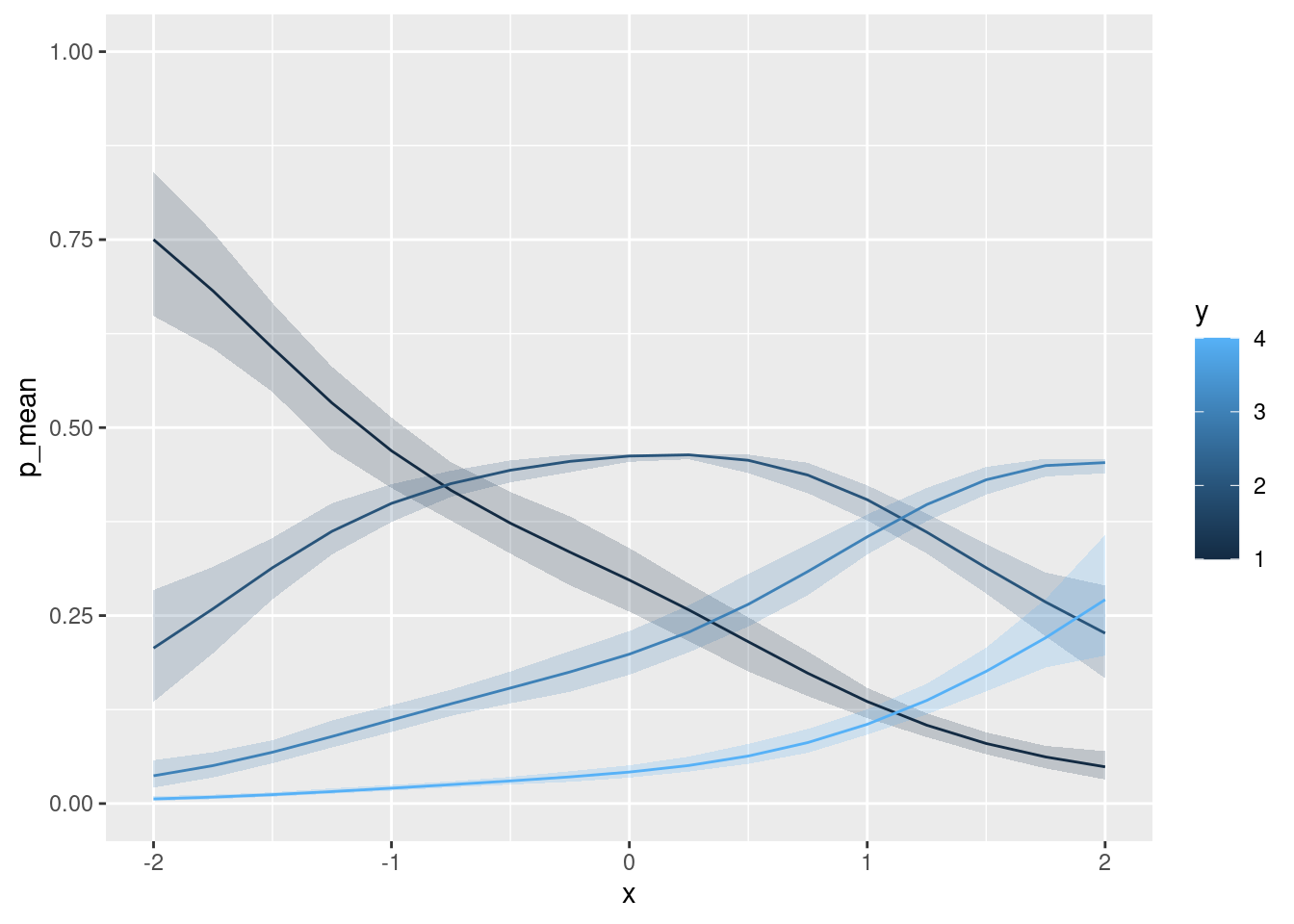
Distributional regression in mgcv
?family.mgcv
gaulss
n <- 500
set.seed(123)
df <- data.frame(x = runif(n))
df$y <- rnorm(n = n, mean = x, sd = .1 * exp(x))
ggplot(data = df, aes(x = x, y = y)) +
  geom_point()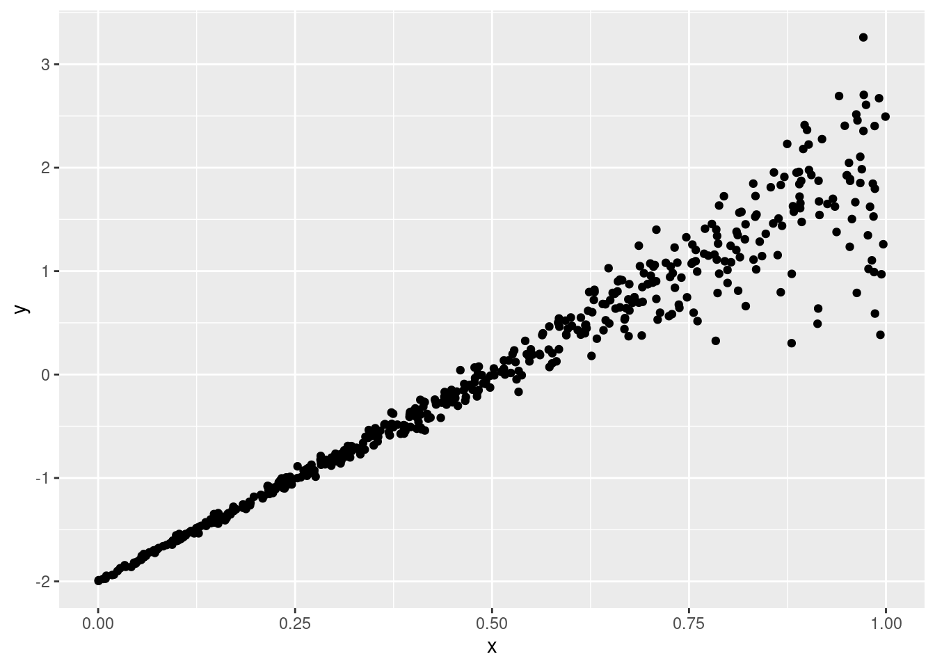
m <- gam(list(y ~ s(x), ~ s(x)),
         data = df, family = gaulss())
plot(m, pages = 1)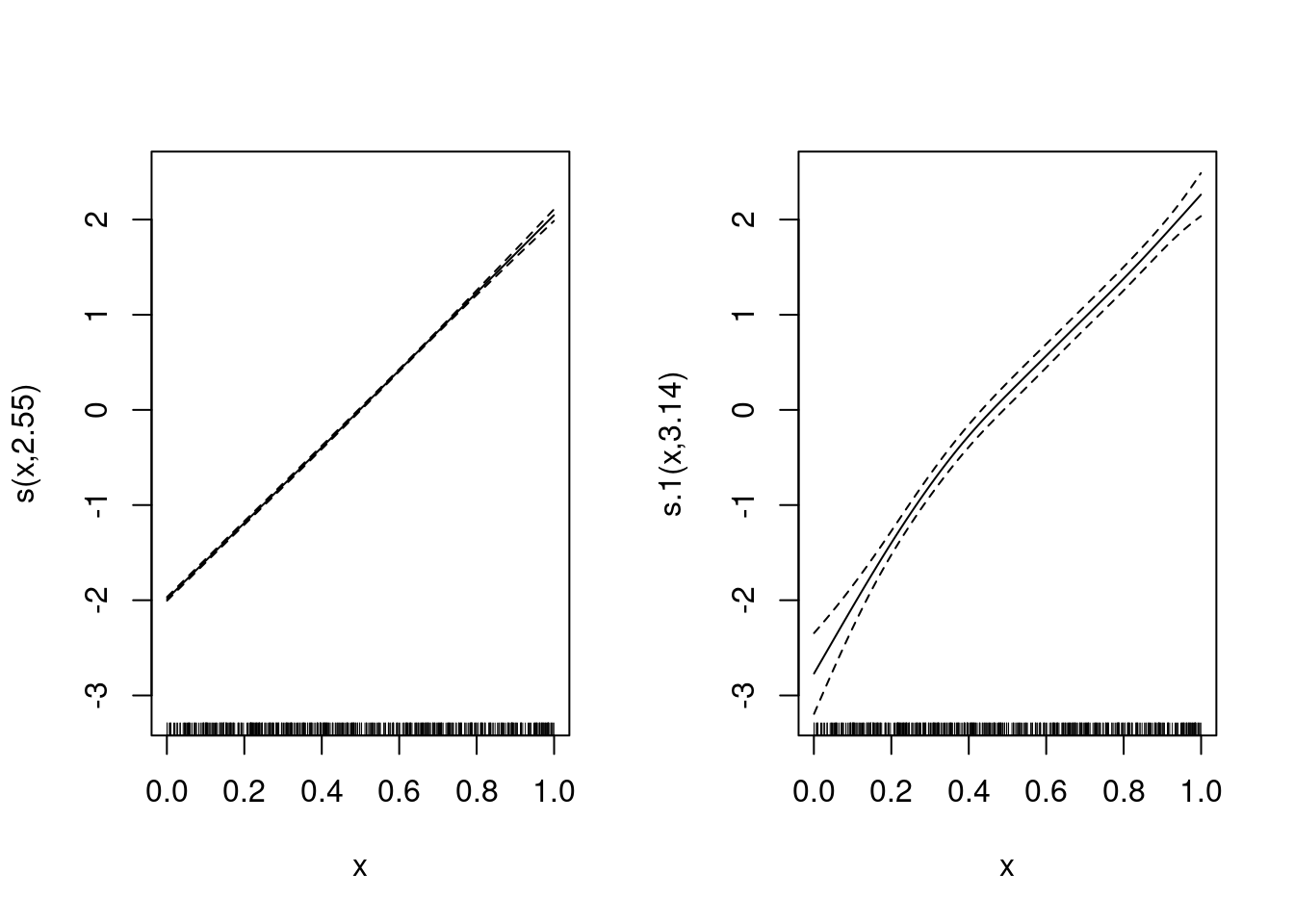
nd <- data.frame(x = seq(0, 1, by = .1))
nd$mu <- predict(m, newdata = nd, type = "link")[, 1]
nd$sigma <- exp(predict(m, newdata = nd, type = "link")[, 2]) + .01
ggplot(data = df, aes(x = x)) +
  geom_point(aes(y = y)) +
  geom_line(data = nd, aes(y = mu)) +
  geom_line(data = nd, aes(y = qnorm(p = .1, mean = mu, sd = sigma)), linetype = "dashed") +
  geom_line(data = nd, aes(y = qnorm(p = .9, mean = mu, sd = sigma)), linetype = "dashed")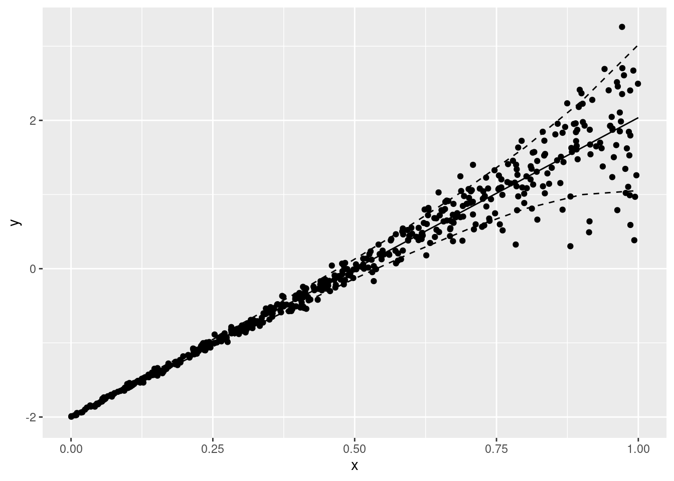
ziplss
?ziplss
set.seed(123)
n <- 1000
x <- runif(n)
eta1 <- x
eta2 <- 2*x
p <- 1 - exp(-exp(eta1)) ## cloglog link
y <- as.numeric(runif(n)<p) ## 1 for presence, 0 for absence
plot(x, y)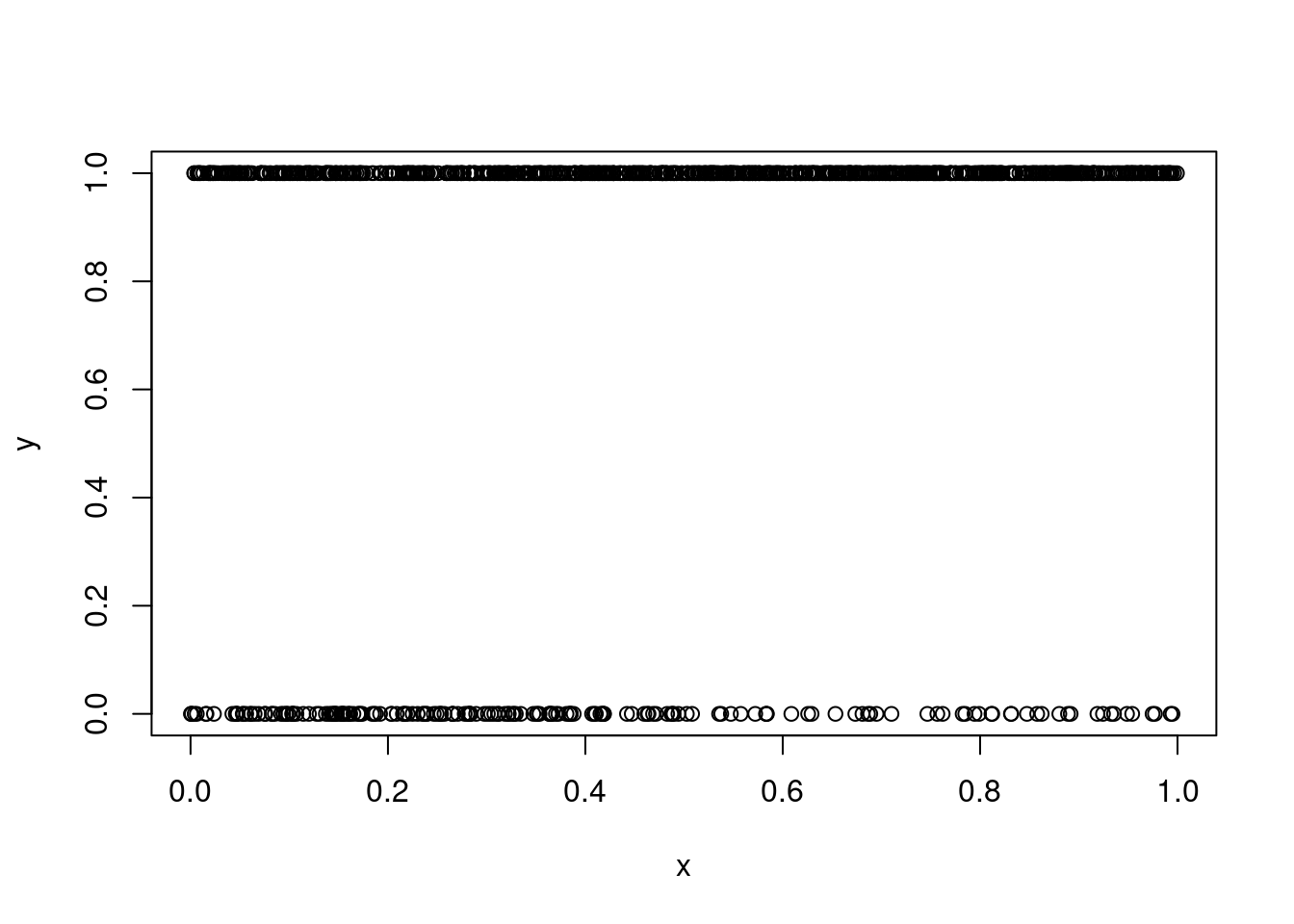
table(y)y
0 1
191 809 ind <- y > 0
p <- ppois(q = 0, lambda = exp(eta2[ind]))
y[ind] <- qpois(p = runif(sum(ind), p, 1), lambda = exp(eta2[ind]))
table(y[ind])
  1   2   3   4   5   6   7   8   9  10  11  12  14
170 167 149 106 62 54 39 21 17 14 6 1 3 plot(x, y)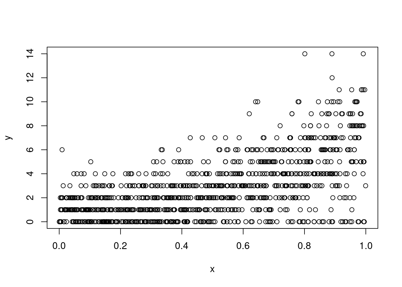
b <- gam(list(y ~ x, ~ x), family = ziplss())
plot(b, pages = 1, all.terms = T)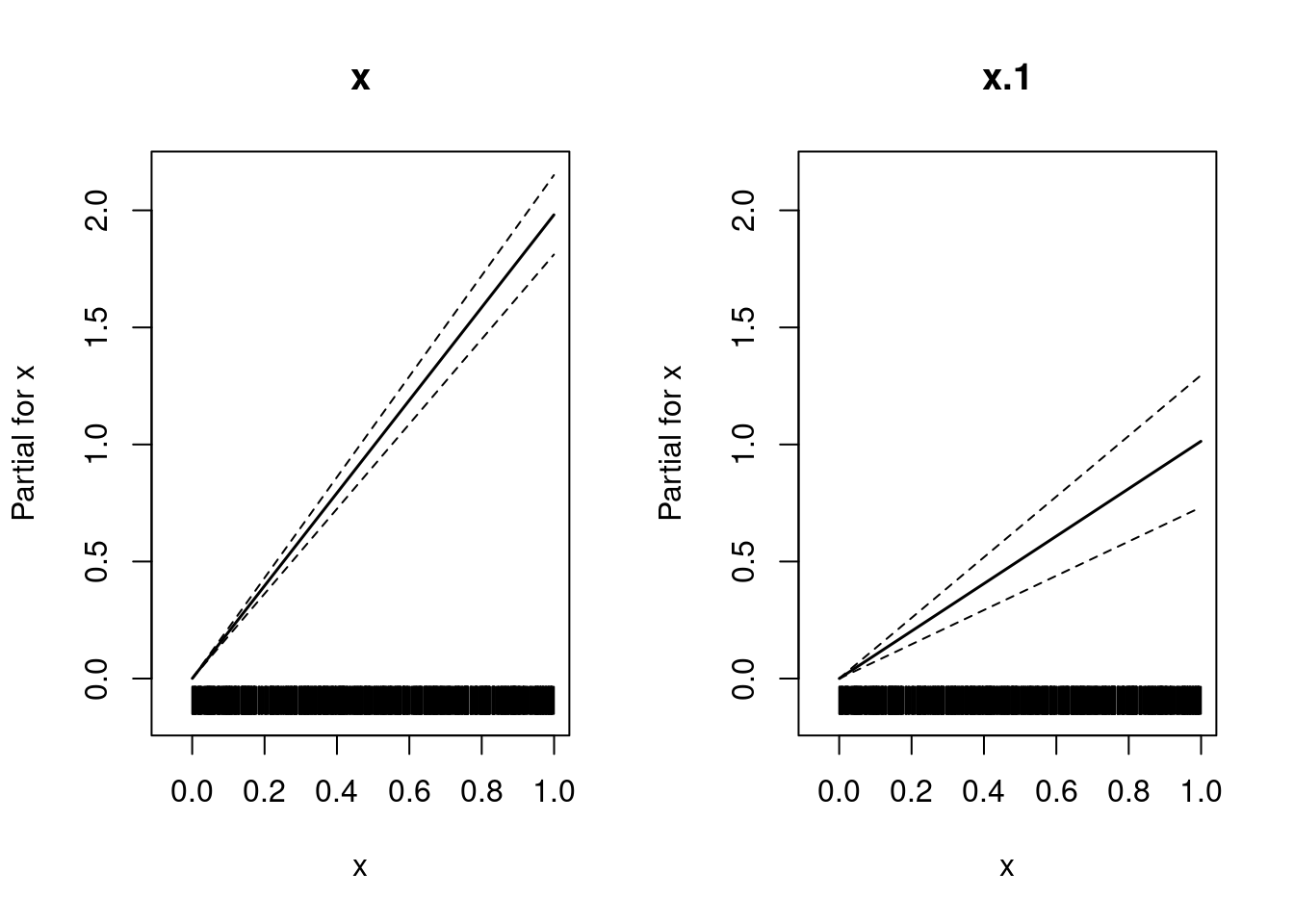
References
Allaire, J. J., Teague, C., Scheidegger, C., Xie, Y., & Dervieux, C. (2024). Quarto (Version 1.4.553). https://doi.org/10.5281/zenodo.5960048
Bürkner, P.-C. (2017). Brms: An R Package for Bayesian Multilevel Models Using Stan. Journal of Statistical Software, 80, 1–28. https://doi.org/10.18637/jss.v080.i01
Bürkner, P.-C. (2018). Advanced Bayesian Multilevel Modeling with the R Package brms. The R Journal, 10(1), 395–411.
Carpenter, B., Gelman, A., Hoffman, M. D., Lee, D., Goodrich, B., Betancourt, M., Brubaker, M., Guo, J., Li, P., & Riddell, A. (2017). Stan: A Probabilistic Programming Language. Journal of Statistical Software, 76, 1–32. https://doi.org/10.18637/jss.v076.i01
Gelman, A., & Su, Y.-S. (2024). Arm: Data analysis using regression and multilevel/hierarchical models. https://CRAN.R-project.org/package=arm
R Core Team. (2024). R: A Language and Environment for Statistical Computing (Version 4.4.1). R Foundation for Statistical Computing.
Wickham, H. (2016). ggplot2: Elegant graphics for data analysis. Springer-Verlag New York. https://ggplot2.tidyverse.org