All contents are licensed under CC BY-NC-ND 4.0.

1 Working with ‘real’ data

R is a powerful tool, not only for analysis, but also for managing data.

1.1 Reproducible data management

Avoid any steps in spreadsheet-software as MS Excel that are done ‘by hand’, and that are non-reproducible.
Workflow A:
- Generate an R-Script 01_datamanagement.R that loads your data and does all the steps, and returns an object df that is used for any further steps.
- Run this file using source(01_datamanagement.R).
Workflow B: Generate a markdown file that not only does the above, but also documents all your steps (A brief intro to markdown in Session 05).

1.2 Preparatory steps prior R

Data management in R begins with loading the data into R. But before we think about the technical way in which we read our data into R, we should first ensure that they are ‘prepared’ for this import. If we neglect a few basic rules in this preparatory work, we actually only hold back problems (for which we then only have to find unnecessarily ‘complicated’ solutions in R).

The first line of the data frame is reserved for the variable names: If we set header = TRUE (R functionsread.csv ()orread.table ()) the first line in the data frame becomes for the variable names recycled.
The first column(s) should be used to define the observation unit: Tree ID (, plot ID, …). Prefer to keep this information separate: combining several variables (in R) is easier than splitting one variable into several variables.

1.3 Variable names

Avoid variable names, values, or cells with spaces. If ignored – and not adequately handled during data import – each word is treated as a (value of) a separate variable. This leads to errors that are always related to the fact that the number of elements varies between the lines (matrix ‘behavior’ of the data frame).
If several words are to be put together, ideally use underscores, eg. Count_per_ha (Alternatively, you can also use dots – Count.per.ha –, or start every single word with a capital letter – CountPerHa).
Decide on a rule and try to stick to it!
Functions like tolower,gsub ()andstringsplit are useful helpers to quickly carry out repairs in R.
Make sure that all missing values – especially empty cells – are marked with NA.
Delete all free text comments (this only leads to extra columns or an inflation of NAs).

1.4 Preparatory Work in R

Before reading in a data frame, you have to tell R where the file can be found.

To achieve this, it can be helpful to find out which working directory R is currently accessing:

getwd()

If different from the storage location of the data frame, we have to change this working directory:

setwd("<Path of the folder in which the data file is saved>")

By executing this function call, R now knows in which working directory we want to work.

For RStudio users

It is very helpful to save the current .R code file and the data frame in the same directory: At the beginning of a working session, you can then click on Session $\rightarrow$ Set Working Directory $\rightarrow$ To Source File Location (this also facilitates collaboration).

Spreadsheet software (such as MS Excel) allows data frames to be saved in many different file formats:

The most popular non-standard formats (i.e. not .xls or.xlsx) to save a data frame are .csv (for comma-separated value) and.txt (tab-separated text file).
Depending on this choice, a line’s contents are either separated by commas or tabs (referred to as ‘separation argument’).
Attention: Under operating systems with German language setting, commas are the default setting for the argument to represent decimal numbers. Here it is necessary to change the default values for the arguments sep anddec to sep = "; " and dec = ", " (required in read.table(), read.csv() and read.csv2(); see also the next sections).

1.5 `read.table()`

If the data was saved in the above-mentioned tab-separated text format .txt, the function read.table() is a simple way of importing data:

d <- read.table("<FileName>.txt", header = TRUE)

By previously defining the working directory (setwd ()), the dataser can be imported directly by specifying the file name.
The value of the header argument can be used to determine whether the first line of the dataframe contains the variable names (TRUE is the default value here).
The separation argument sep is set to the value "", since the read.table command is defined for tab-separated text formats.

To specify a different separation argument, the value of the argument sep must be changed:

df <- read.table("<FileName>.txt", header = FALSE, sep = ";")

1.6 `read.csv()` and `read.csv2()`

The functions read.csv() and read.csv2() can be used to read data files in .csv (Comma Separated Values) format.

.csv dataframes can be easily imported into R and are therefore a preferred format.
read.csv() and read.csv2() use different separation arguments: for read.csv() the comma, for read.csv2() the semicolon (open your data frame in a text editor in order to quickly find out your separation argument).
read.csv() and read.csv2() are special cases of read.table(): This means that the arguments for read.table() can alternately also be used for read.csv() and read.csv2().
read.csv() and read.csv2() are very similar to read.table() and differ from read.table() in only three aspects:
- The separation argument sep,
- he argument header is always set toTRUE, and
- the argument fill is also TRUE, which means that if lines have unequal lengths, read.csv() and read.csv2() will always fill the short lines with empty cells.

d <- read.csv("data.csv", header = T, sep = ";", dec = ",", stringsAsFactor = F)
names(d)

1.7 Factors

Working with factors:

In recent R versions, data imports with stringsAsFactor = FALSE as default, which is good:

Check the structure of the data frame with the help of str(): Were variables imported as strings (class chr) and not as numeric (class num) as expected? If so, check the characteristics of these variables for incorrect values with unique() or xtabs().
Also check with unique() or xtabs() the characteristics of the variables that were planned to be read in as chr: Typing errors can easily lurk here as well.
Use df$var <- as.factor(df$var) to finally assign the factor class to variable var.

1.8 `attach`, `subset` and `merge`

Never say never but never use attach().

… use a short name for the data frame object (e.g. df) to keep typing to a minimum!

The function merge(data_set1, data_set2, by, ...) can be used to link two data frames using a key variable:

library("plyr")
dd <- ddply(drought, c("species"), summarize,
            mean_bair = mean(bair),
            sd_bair = sd(bair),
            mean_elev = mean(elev),
            sd_elev = sd(elev))
head(merge(drought, dd, by = c("species")))

##   species  bair  elev mean_bair   sd_bair mean_elev  sd_elev
## 1   Beech 0.697 475.0 0.8152727 0.2159037  804.3182 277.0922
## 2   Beech 0.606 480.0 0.8152727 0.2159037  804.3182 277.0922
## 3   Beech 0.718 507.5 0.8152727 0.2159037  804.3182 277.0922
## 4   Beech 0.480 580.0 0.8152727 0.2159037  804.3182 277.0922
## 5   Beech 0.822 750.0 0.8152727 0.2159037  804.3182 277.0922
## 6   Beech 0.944 780.0 0.8152727 0.2159037  804.3182 277.0922

subset can be used to split a dataframe according to the result of a logical comparison:

(tmp <- range(drought$elev %/% 250))

## [1] 1 6

br <- seq(tmp[1] * 250, (tmp[2] + 1) * 250, by = 250)
drought$elev_cut <- cut(drought$elev, breaks = br)
sdf <- subset(drought, elev_cut == "(500,750]" & species == "Beech")
sdf

##     bair  elev species  elev_cut
## 26 0.718 507.5   Beech (500,750]
## 27 0.480 580.0   Beech (500,750]
## 28 0.822 750.0   Beech (500,750]

2 Descriptive analysis for univariate samples

2.1 Continuously scaled variable

2.1.1 Location

mean, weighted.mean
median, quantile (calculates percentiles probs = seq(0, 1, by = .01), and quartiles for probs = c(.25, .5, .75))
summary (returns: min, 1st quartile, median, mean, 3rd quartile, max)

2.1.2 Exercises

drought$species <- as.factor(drought$species)
## mean:
mean(drought$bair)
## weighted mean:
tmp <- nrow(drought)/table(drought$species)
tmp <- data.frame(species = factor(levels(drought$species), levels = levels(drought$species)), 
                  w = as.numeric(tmp))
tmp <- merge(drought[, c("species", "bair")], tmp, by = "species")
tmp$w <- tmp$w/sum(tmp$w)
aggregate(x = tmp[, c("w")], by = list(tmp$species), FUN = sum)
weighted.mean(tmp$bair, w = tmp$w)
rm(tmp)
## median:
median(drought$bair)
## quartiles:
quantile(drought$bair, probs = c(.25, .5, .75))
## summary:
summary(drought$bair)

Mode: A sample of a continuously scaled variable doesn’t have a mode:

library("ggplot2")
ggplot(data = drought, aes(x = bair)) + 
  geom_rug()

# plot(table(drought$bair), las = 2, bty = "n")

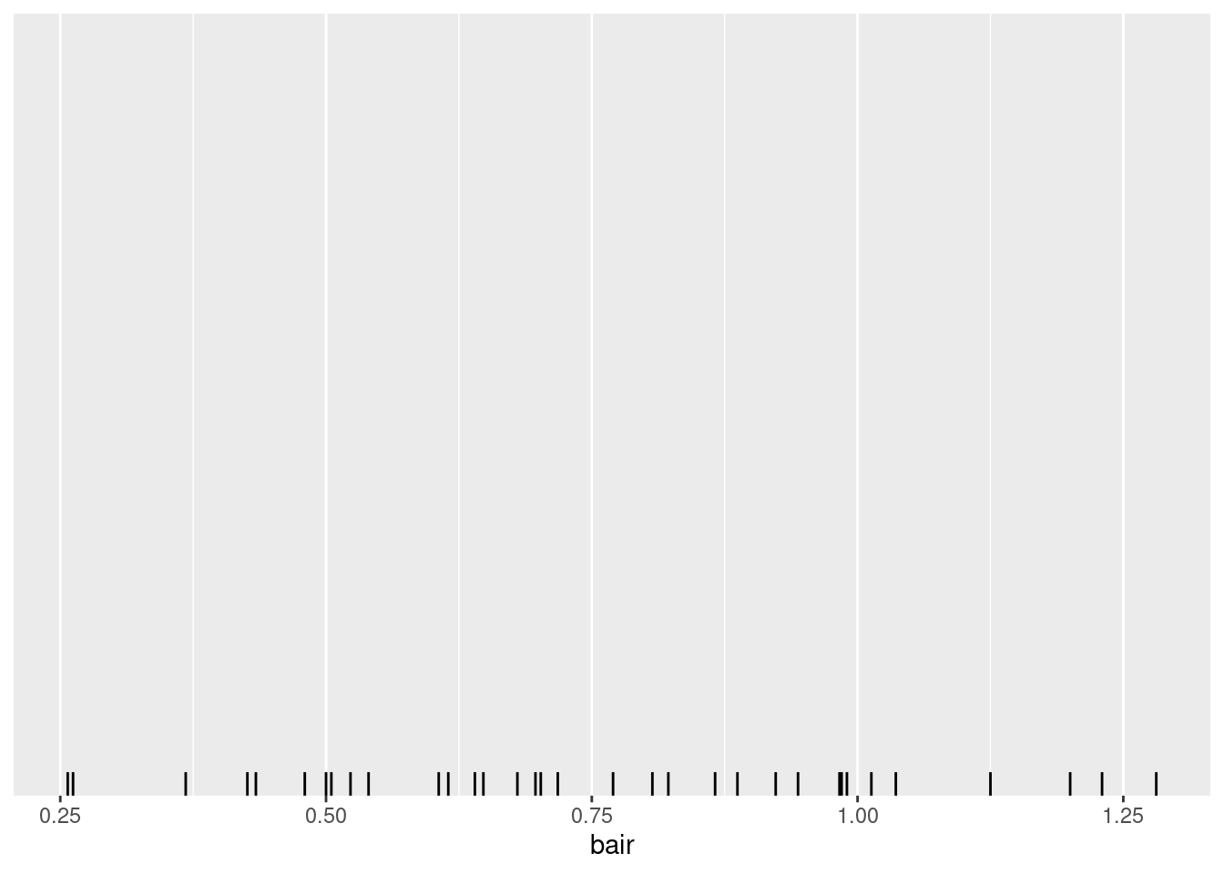
… but the density of such a variable might have a maximum. So we cannot calculate a mode, but with using techniques such as kernel density estimation – ggplot-geom geom_density – the location of the maximum density can be estimated.

p <- ggplot(data = drought, aes(x = bair)) + 
  geom_density()
gp <- ggplot_build(p)
x_at_max_y <- gp$data[[1]]$x[which.max(gp$data[[1]]$density)]
p + geom_vline(xintercept = x_at_max_y, linetype = "dashed")

2.1.3 Scale / variation

Methods to describe the scale / variation:

range (calculates min and max)
var (variance)
sd (standard deviation)
mad (‘median absolute deviation’, function mad(x) is just a more general implementation of median(abs(x - median(x))))
IQR (interquartile range)

Argument na.rm = TRUE removes all missing values in advance!

2.1.4 Exercises

x <- drought$bair
mad

## function (x, center = median(x), constant = 1.4826, na.rm = FALSE, 
##     low = FALSE, high = FALSE) 
## {
##     if (na.rm) 
##         x <- x[!is.na(x)]
##     n <- length(x)
##     constant * if ((low || high) && n%%2 == 0) {
##         if (low && high) 
##             stop("'low' and 'high' cannot be both TRUE")
##         n2 <- n%/%2 + as.integer(high)
##         sort(abs(x - center), partial = n2)[n2]
##     }
##     else median(abs(x - center))
## }
## <bytecode: 0x57d260503bc8>
## <environment: namespace:stats>

c(mad(x, constant = 1),
  median(abs(x - median(x))),
  sd(x),
  var(x),
  IQR(x))

## [1] 0.21150000 0.21150000 0.27400800 0.07508039 0.44600000

2.2 Categorically scaled variables

table as ‘standard function’ for absolute frequency distribution, xtabs as an alternative with formula syntax (and labeling with variable names if table is created from data set).

… while preparing, this section somehow got longer and longer. For a general introduction to R, at some point, when you feel like it, just move on to next section on bivariate sample.

2.2.1 One dimensional:

table(drought$species)

## 
##  Beech Spruce 
##     11     23

xtabs(~ drought$species)

## drought$species
##  Beech Spruce 
##     11     23

xtabs(~ species, data = drought)

## species
##  Beech Spruce 
##     11     23

addNA and useNA show slightly different behavior:

tmp <- as.factor(c(as.character(drought$species), NA))
table(tmp)

## tmp
##  Beech Spruce 
##     11     23

table(drought$species, useNA = "ifany")

## 
##  Beech Spruce 
##     11     23

table(tmp, useNA = "ifany")

## tmp
##  Beech Spruce   <NA> 
##     11     23      1

table(drought$species, useNA = "always")

## 
##  Beech Spruce   <NA> 
##     11     23      0

table(tmp, useNA = "always")

## tmp
##  Beech Spruce   <NA> 
##     11     23      1

xtabs(~ drought$species, addNA = TRUE)

## drought$species
##  Beech Spruce 
##     11     23

xtabs(~ tmp, addNA = T)

## tmp
##  Beech Spruce   <NA> 
##     11     23      1

Visualisation:

ggplot(data = as.data.frame(xtabs(~ species, data = drought))) + 
  geom_point(aes(x = species, y = Freq)) + 
  expand_limits(y = 0)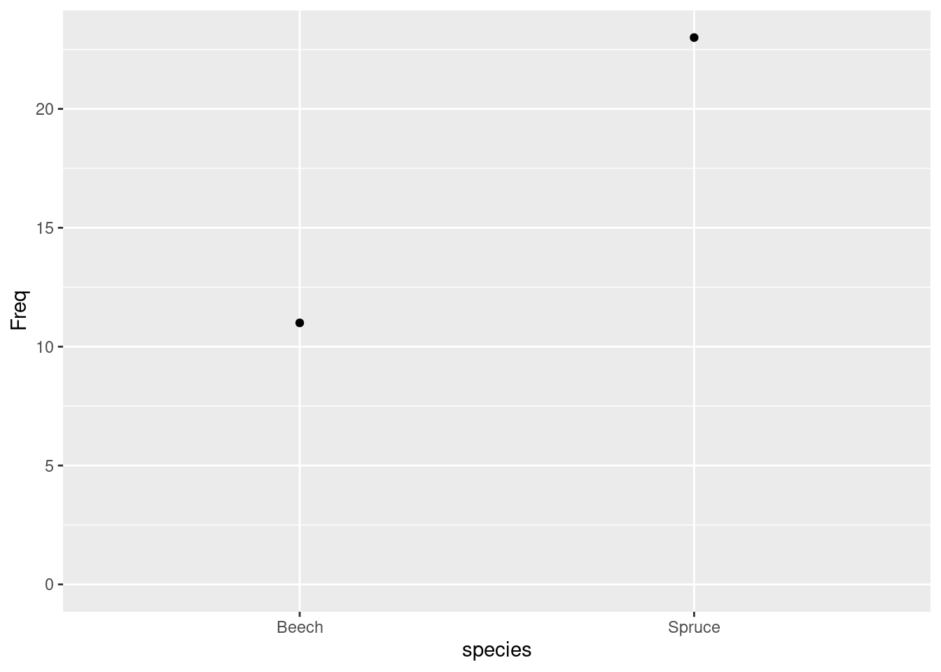

2.2.2 Two dimensional

… this illustrational example shows bad scientific practice since we cut continuous variables into binary categories, and by this bin a lot of valuable information!

tmp <- data.frame(species = drought$species)
tmp$elevation <- cut(drought$elev, breaks = sort(c(range(drought$elev), 1000)), include.lowest = T, dig.lab = 4)
tmp$bair <- cut(drought$bair, breaks = sort(c(range(drought$bair), 1)), include.lowest = T)
table(tmp$bair, tmp$elevation) ##  ... (a bit) lost.

##            
##             [335,1000] (1000,1540]
##   [0.257,1]         19           9
##   (1,1.28]           0           6

xtabs(~ bair + elevation, data = tmp) ## ... with variable name labels!

##            elevation
## bair        [335,1000] (1000,1540]
##   [0.257,1]         19           9
##   (1,1.28]           0           6

Default plot (see add-on package ggmosaic for a ggplot alternative):

xtabs(~ bair + elevation, data = tmp) ## Labels!

##            elevation
## bair        [335,1000] (1000,1540]
##   [0.257,1]         19           9
##   (1,1.28]           0           6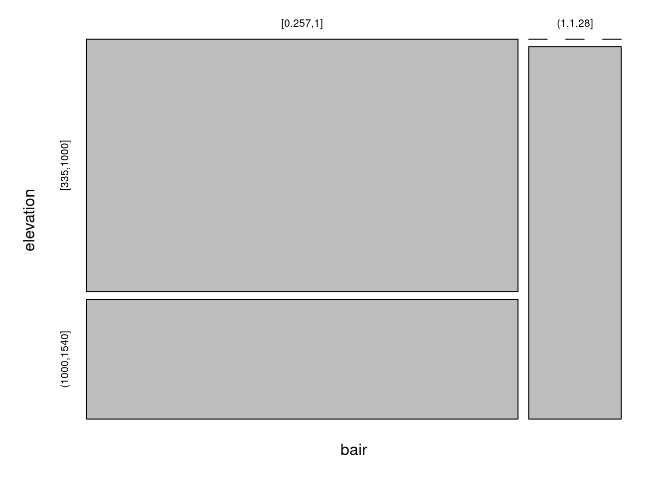

par(mfrow = c(1, 1), mar = c(3, 3, 1, 1))
plot(xtabs(~ bair + elevation, data = tmp), main = "")

# install.packages("ggmosaic")
library("ggmosaic")
ggplot(data = tmp) +
  geom_mosaic(aes(x = product(elevation, bair), 
                  fill = elevation))

## Warning: The `scale_name` argument of `continuous_scale()` is deprecated as of ggplot2
## 3.5.0.
## This warning is displayed once every 8 hours.
## Call `lifecycle::last_lifecycle_warnings()` to see where this warning was
## generated.

## Warning: The `trans` argument of `continuous_scale()` is deprecated as of ggplot2 3.5.0.
## ℹ Please use the `transform` argument instead.
## This warning is displayed once every 8 hours.
## Call `lifecycle::last_lifecycle_warnings()` to see where this warning was
## generated.

## Warning: `unite_()` was deprecated in tidyr 1.2.0.
## ℹ Please use `unite()` instead.
## ℹ The deprecated feature was likely used in the ggmosaic package.
##   Please report the issue at <https://github.com/haleyjeppson/ggmosaic>.
## This warning is displayed once every 8 hours.
## Call `lifecycle::last_lifecycle_warnings()` to see where this warning was
## generated.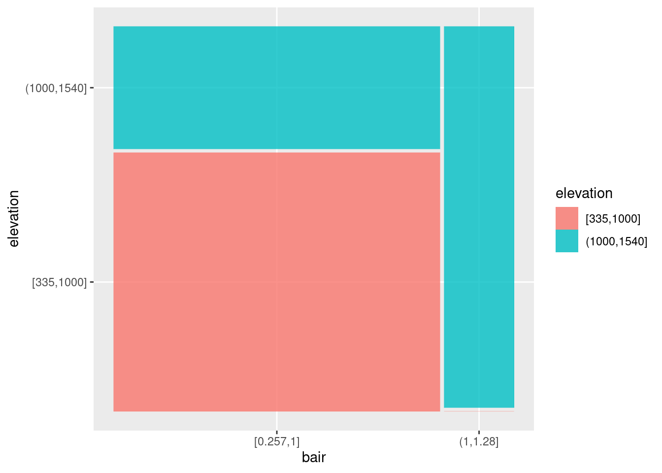

2.2.3 `addmargins`, `margin.table`, and `prop.table`

One dimensional:

addmargins(table(tmp$bair))

## 
## [0.257,1]  (1,1.28]       Sum 
##        28         6        34

margin.table(table(tmp$bair))

## [1] 34

prop.table(table(tmp$bair))

## 
## [0.257,1]  (1,1.28] 
## 0.8235294 0.1764706

margin.table(prop.table(table(tmp$bair)))

## [1] 1

Two dimensional:

addmargins(table(tmp$elevation, tmp$bair))

##              
##               [0.257,1] (1,1.28] Sum
##   [335,1000]         19        0  19
##   (1000,1540]         9        6  15
##   Sum                28        6  34

margin.table(table(tmp$elevation, tmp$bair))

## [1] 34

margin.table(table(tmp$elevation, tmp$bair), margin = 1)

## 
##  [335,1000] (1000,1540] 
##          19          15

margin.table(table(tmp$elevation, tmp$bair), margin = 2)

## 
## [0.257,1]  (1,1.28] 
##        28         6

prop.table(table(tmp$elevation, tmp$bair))

##              
##               [0.257,1]  (1,1.28]
##   [335,1000]  0.5588235 0.0000000
##   (1000,1540] 0.2647059 0.1764706

prop.table(table(tmp$elevation, tmp$bair), margin = 1)

##              
##               [0.257,1] (1,1.28]
##   [335,1000]        1.0      0.0
##   (1000,1540]       0.6      0.4

prop.table(table(tmp$elevation, tmp$bair), margin = 2)

##              
##               [0.257,1]  (1,1.28]
##   [335,1000]  0.6785714 0.0000000
##   (1000,1540] 0.3214286 1.0000000

margin.table(prop.table(table(tmp$elevation, tmp$bair)))

## [1] 1

addmargins(prop.table(table(tmp$elevation, tmp$bair)))

##              
##               [0.257,1]  (1,1.28]       Sum
##   [335,1000]  0.5588235 0.0000000 0.5588235
##   (1000,1540] 0.2647059 0.1764706 0.4411765
##   Sum         0.8235294 0.1764706 1.0000000

addmargins(prop.table(table(tmp$elevation, tmp$bair), margin = 1))

##              
##               [0.257,1] (1,1.28] Sum
##   [335,1000]        1.0      0.0 1.0
##   (1000,1540]       0.6      0.4 1.0
##   Sum               1.6      0.4 2.0

addmargins(prop.table(table(tmp$elevation, tmp$bair), margin = 2))

##              
##               [0.257,1]  (1,1.28]       Sum
##   [335,1000]  0.6785714 0.0000000 0.6785714
##   (1000,1540] 0.3214286 1.0000000 1.3214286
##   Sum         1.0000000 1.0000000 2.0000000

addmargins(prop.table(table(tmp$elevation, tmp$bair), margin = 1), margin = 2)

##              
##               [0.257,1] (1,1.28] Sum
##   [335,1000]        1.0      0.0 1.0
##   (1000,1540]       0.6      0.4 1.0

addmargins(prop.table(table(tmp$elevation, tmp$bair), margin = 2), margin = 1)

##              
##               [0.257,1]  (1,1.28]
##   [335,1000]  0.6785714 0.0000000
##   (1000,1540] 0.3214286 1.0000000
##   Sum         1.0000000 1.0000000

2.2.4 Applied example

## Session 03:
overlap_seq <- function(x, delta) {
  tmp <- x %/% delta
  tmp2 <- x %% delta
  if (tmp2[which.max(x)] == 0) {
    result <- delta * (min(tmp, na.rm = T):max(tmp, na.rm = T))
  } else {
    result <- delta * (min(tmp, na.rm = T):(max(tmp, na.rm = T) + 1))
  }
  return(result)
}
tmp$elevCut <- cut(drought$elev, breaks = overlap_seq(x = drought$elev, delta = 250), dig.lab = 4)
tmp$bairCut <- cut(drought$bair, breaks = overlap_seq(x = drought$bair, delta = .25))
(xtab <- xtabs(~ elevCut + bairCut + species, data = tmp))

## , , species = Beech
## 
##              bairCut
## elevCut       (0.25,0.5] (0.5,0.75] (0.75,1] (1,1.25] (1.25,1.5]
##   (250,500]            0          2        0        0          0
##   (500,750]            1          1        1        0          0
##   (750,1000]           0          0        2        0          0
##   (1000,1250]          0          1        1        2          0
##   (1250,1500]          0          0        0        0          0
##   (1500,1750]          0          0        0        0          0
## 
## , , species = Spruce
## 
##              bairCut
## elevCut       (0.25,0.5] (0.5,0.75] (0.75,1] (1,1.25] (1.25,1.5]
##   (250,500]            0          3        0        0          0
##   (500,750]            4          1        1        0          0
##   (750,1000]           1          1        1        0          0
##   (1000,1250]          1          2        2        1          1
##   (1250,1500]          0          0        1        2          0
##   (1500,1750]          0          0        1        0          0

round(100 * addmargins(prop.table(xtab, margin = c(1, 3))), 2)[, , "Beech"]

##              bairCut
## elevCut       (0.25,0.5] (0.5,0.75] (0.75,1] (1,1.25] (1.25,1.5]    Sum
##   (250,500]         0.00     100.00     0.00     0.00       0.00 100.00
##   (500,750]        33.33      33.33    33.33     0.00       0.00 100.00
##   (750,1000]        0.00       0.00   100.00     0.00       0.00 100.00
##   (1000,1250]       0.00      25.00    25.00    50.00       0.00 100.00
##   (1250,1500]                                                          
##   (1500,1750]                                                          
##   Sum

round(100 * addmargins(prop.table(xtab, margin = c(1, 3))), 2)[, , "Spruce"]

##              bairCut
## elevCut       (0.25,0.5] (0.5,0.75] (0.75,1] (1,1.25] (1.25,1.5]    Sum
##   (250,500]         0.00     100.00     0.00     0.00       0.00 100.00
##   (500,750]        66.67      16.67    16.67     0.00       0.00 100.00
##   (750,1000]       33.33      33.33    33.33     0.00       0.00 100.00
##   (1000,1250]      14.29      28.57    28.57    14.29      14.29 100.00
##   (1250,1500]       0.00       0.00    33.33    66.67       0.00 100.00
##   (1500,1750]       0.00       0.00   100.00     0.00       0.00 100.00
##   Sum             114.29     178.57   211.90    80.95      14.29 600.00

par(mfrow = c(1, 1), mar = c(0, 0, 0, 0) + .1)
plot(xtabs(~ species + elevCut + bairCut, data = tmp), las = 2, off = 5, main = "", 
     col = colorspace::divergingx_hcl(n = length(levels(tmp$bairCut)), rev = T))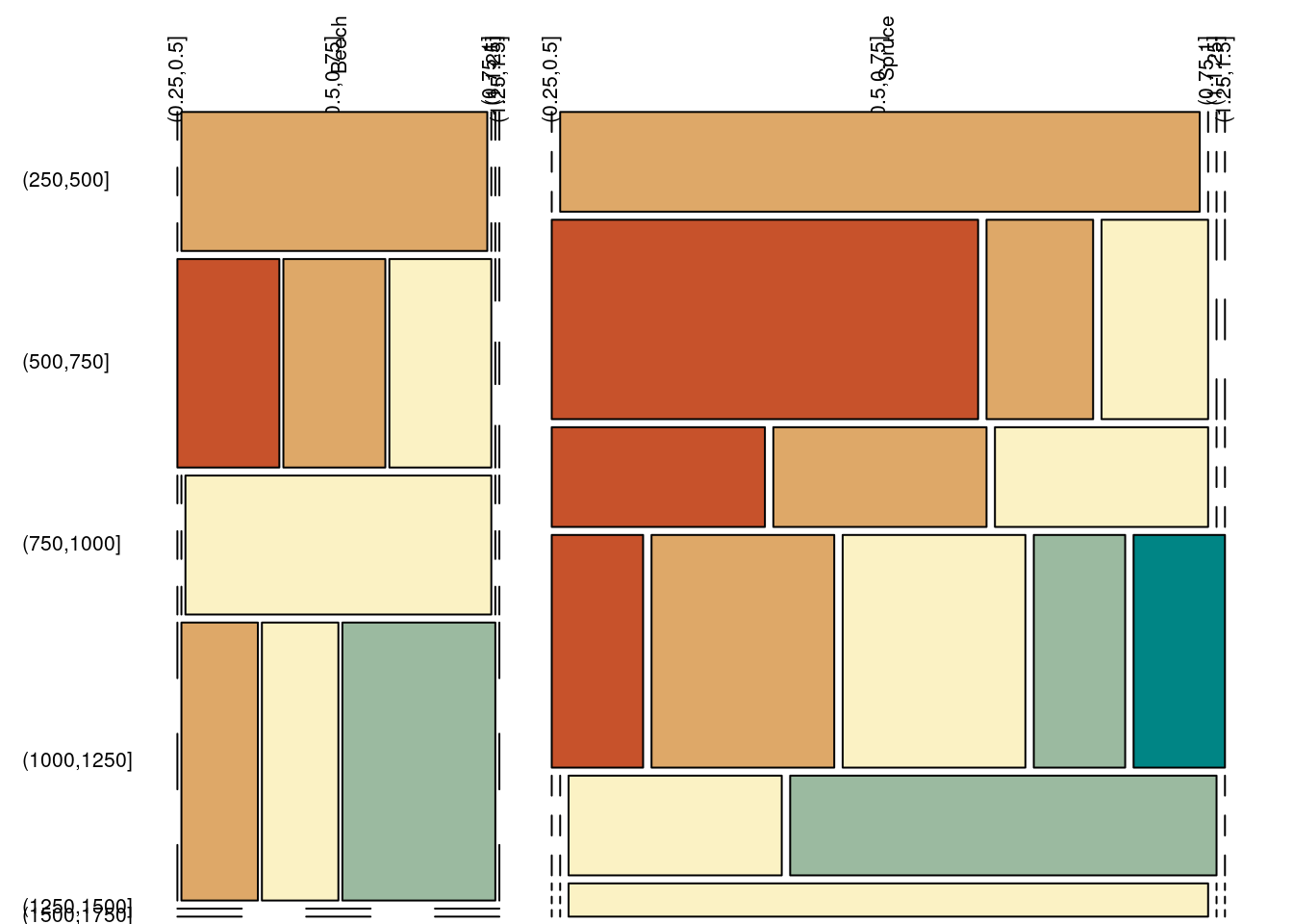

2.2.5 Mode

(xtab <- xtabs(~ species + elevCut + bairCut, data = tmp))
sort(xtab, decreasing = TRUE)[1]
which(xtab == max(xtab), arr.ind = TRUE)
xtab[2, 2, 1]

3 Bivariate samples

A bivariate sample is a set of observation units, for which each has two characteristics that have been measured.

set.seed(123)
A <- matrix(nrow = 5, ncol = 5, data = runif(25))
A[, 1:2]

##           [,1]      [,2]
## [1,] 0.2875775 0.0455565
## [2,] 0.7883051 0.5281055
## [3,] 0.4089769 0.8924190
## [4,] 0.8830174 0.5514350
## [5,] 0.9404673 0.4566147

pmax(A[, 1], A[, 2]) ## parallel maxima

## [1] 0.2875775 0.7883051 0.8924190 0.8830174 0.9404673

cor for correlation coefficient,
cov for (variance) covariance (matrix).

x <- drought$bair
y <- drought$elev/1000
cor(x, y, method = "pearson")

## [1] 0.6174439

cov(cbind(x, y))

##            x          y
## x 0.07508039 0.05579038
## y 0.05579038 0.10874194

c(cov(x, y), var(x), var(y))

## [1] 0.05579038 0.07508039 0.10874194

4 Probability distribution models

4.1 Definitions for continuous random variables:

Random variable $X\in\mathbf{R}$ follows distribution $F$ with density $f(x)\geq0\,\forall x\in\mathbf{R}$
Cumulative density function $F(x)=\int\limits_{-\infty}^{x}{f(z)}\text{d}z$, with $F(-\infty)=0$ and $F(\infty)=1$.
Quantile function $Q(x)=F^{-1}(x)$

Implementation in R: code + distribution abbreviation

Code	meaning
`d`	density
`p`	cdf (probability)
`q`	quantile
`r`	random number generation

4.2 Distribution models for continuous random variables:

Distribution	Abbreviation	Parameter	Wiki
Continuous uniform	`unif`	`min`, `max`	Link
Normal (aka. Gaussian)	`norm`	`mean`, `sd`	Link
Lognormal	`lnorm`	`meanlog`, `sdlog`	Link
Exponential	`exp`	`rate`	Link
Beta	`beta`	`shape1`, `shape2`	Link
Chi-squared	`chisq`	`df`, `ncp`	Link
F	`f`	`df1`, `df2`, `ncp`	Link
Student-t	`t`	`df`, `ncp`	Link
Gamma	`gamma`	`shape`, `rate`, `scale` = 1/`rate`	Link
Weibull	`weibull`	`shape`, `scale`	Link

N <- 100
set.seed(123)
A <- rbind(data.frame("distribution" = "U[0, 1]", 
                      "value" = runif(n = N, min = 0, max = 1)),
           data.frame("distribution" = "Beta(1/3, 1/3)", 
                      "value" = rbeta(n = N, shape1 = 1/3, shape2 = 1/3)),
           data.frame("distribution" = "N(0, 1)", 
                      "value" = rnorm(n = N, mean = 0, sd = 1)),
           data.frame("distribution" = "t(3)", 
                      "value" = rt(n = N, df = 3, ncp = 0)),
           data.frame("distribution" = "logN(0, 1)", 
                      "value" = rlnorm(n = N, meanlog = 0, sdlog = 1)),
           data.frame("distribution" = "Exp(1)", 
                      "value" = rexp(n = N, rate = 1)),
           data.frame("distribution" = "Chi2(3)", 
                      "value" = rchisq(n = N, df = 3, ncp = 0)),
           data.frame("distribution" = "F(10, 10)", 
                      "value" = rf(n = N, df1 = 10, df2 = 10, ncp = 0)),
           data.frame("distribution" = "Gamma(1, 2)", 
                      "value" = rgamma(n = N, shape = 1, rate = 2)),
           data.frame("distribution" = "Weibull(1, 2)", 
                      "value" = rweibull(n = N, shape = 1, scale = 2)))
ggplot(data = A, aes(x = distribution, y = value)) + 
  geom_boxplot(outliers = F) + 
  geom_jitter()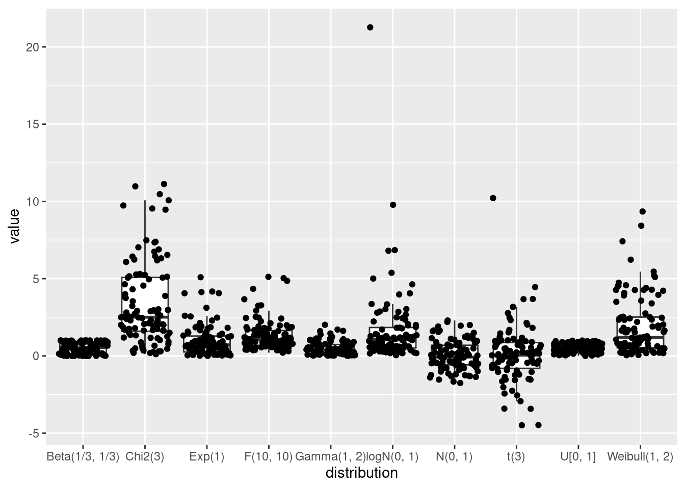

4.3 Distribution models for discrete random variables:

Distribution	Abbreviation	Parameters	Wiki
Binomial	`binom`	`size`, `prob`	Link
Hypergeometric	`hyper`	`m`, `n`,`k`	Link
Negative binomial	`nbinom`	`size`, `prob`,`mu`	Link
Poisson	`pois`	`lambda`	Link
Geometric	`geom`	`prob`	Link
Multinomial	`multinom`	`size`, `prob`	Link

N <- 100
set.seed(123)
A <- rbind(data.frame("distribution" = "Binomial(10, .5)", value = rbinom(n = N, size = 10, prob = .5)),
           data.frame("distribution" = "Hyper(7, 3, 8)", value = rhyper(nn = N, m = 7, n = 3, k = 8)),
           data.frame("distribution" = "NegBin(10, .5)", value = rnbinom(n = N, size = 10, prob = .5)),
           data.frame("distribution" = "Poisson(3)", value = rpois(n = N, lambda = 3)),
           data.frame("distribution" = "Geom(.5)", value = rgeom(n = N, prob = .5)))
ggplot(data = A, aes(x = distribution, y = value)) + 
  geom_boxplot(outliers = F) + 
  geom_jitter()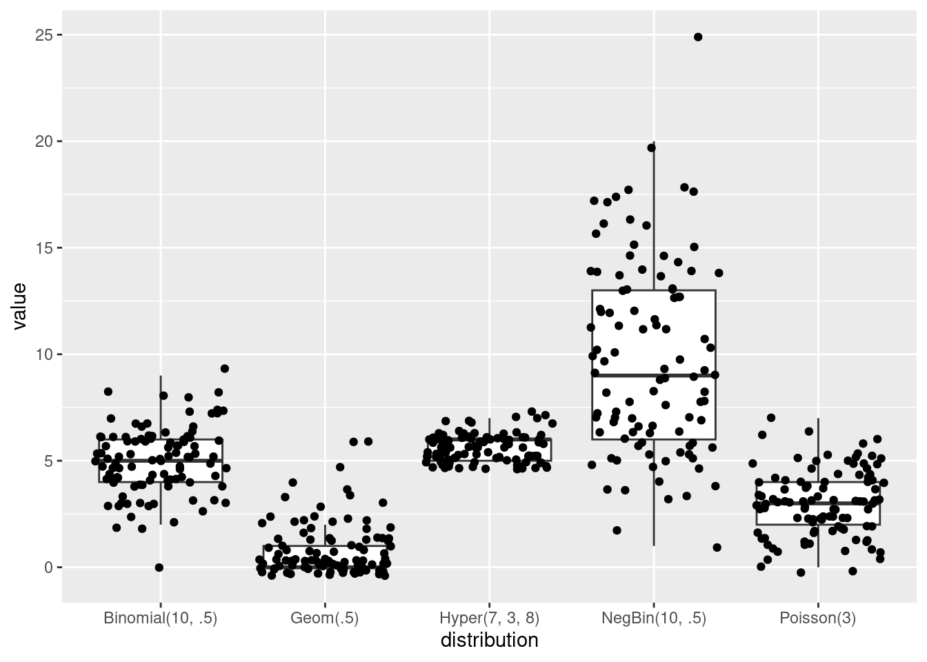

Multinomial:

A <- rmultinom(n = N, size = 10, prob = c(.1, .1, .8))
A <- rbind(data.frame("x" = "1", 
                      "value" = A[1, ]),
           data.frame("x" = "2", 
                      "value" = A[2, ]),
           data.frame("x" = "3", 
                      "value" = A[3, ]))
ggplot(data = A, aes(x = x, y = value)) + 
  geom_boxplot(outliers = F) + 
  geom_jitter()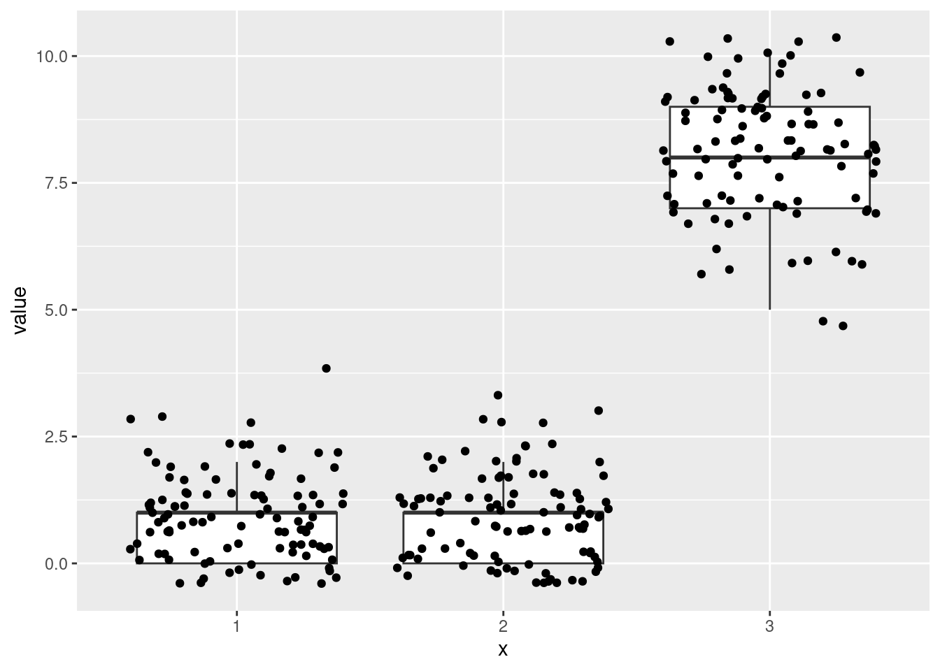

5 Generating ‘random’ numbers

Random numbers are generated in R by an algorithm, they are not real random – whatever this is …
Before a new random number is generated, this algorithm is in a certain state.
The (next) random number depends on this state, drawing this new number alters the state.
RNGkind() lists three character strings for three tasks:
- kind is for draws from the continuous uniform distribution.
- normal.kind is for draws from the normal distribution (I don’t know why there’s this specific kind for the normal, I suppose as the normal distribution is historically so important, there have been algorithms specifically designed for drawing from this distribution …).
- sample.kind for drawing from the diccrete uniform distribution.
Why we won’t have a look on the other algorithms, seeing the idea behind Inversion sampling is really helpful in order to see why being able to generate draws from continuous uniform distribution is already sufficient in order to sample from any other distribution.
Reproducibility is often an important property!
- The state of the random number generating algorithm is initialized by a seed.
- Seeds are generated by system time and session ID (?RNG)

Sys.getpid()

## [1] 7082

(t1 <- Sys.time())

## [1] "2024-06-19 14:27:31 CEST"

(t2 <- Sys.time())

## [1] "2024-06-19 14:27:31 CEST"

t2 - t1

## Time difference of 0.0006723404 secs

We can overwrite thus seed generating by using set.seed():

runif(5)

## [1] 0.44941139 0.76616653 0.02609772 0.19517143 0.88123456

set.seed(123)
runif(5)

## [1] 0.2875775 0.7883051 0.4089769 0.8830174 0.9404673

runif(5)

## [1] 0.0455565 0.5281055 0.8924190 0.5514350 0.4566147

set.seed(123)
runif(5)

## [1] 0.2875775 0.7883051 0.4089769 0.8830174 0.9404673

Generate random numbers using r + distribution abbreviation (uses inversion - sampling)
Random numbers from sets with sample (c (), size, replace = TRUE).

RNGkind()

## [1] "Mersenne-Twister" "Inversion"        "Rejection"

set.seed(1604)
rbinom(5,1,0.5)

## [1] 1 1 1 0 1

rbinom(5,1,0.5)

## [1] 0 1 0 1 0

set.seed(1604)
rbinom(5,1,0.5)

## [1] 1 1 1 0 1

sample(1:10, 5)

## [1] 5 4 1 6 2

sample(1:10, 5, replace = TRUE)

## [1] 10  5  4  5  4

5.1 Inversion-sampling

Inversion sampling is a rather simple application of a mathemcatical thing – the inverse of the cumulative distribution function – that one easily brands as ‘interesting only in mathematical theory’, but which has an incredibly applied value!

Let random variable $X$ have cumulative distribution function $F$.

Let’s assume for the moment we can draw random numbers from this distribution, eg. from the standard normal:

x <- rnorm(1000)

If we plug these into the cumulative distribution function

u <- pnorm(x)
ggplot(data = data.frame(u = u)) + 
  geom_histogram(aes(x = u))

## `stat_bin()` using `bins = 30`. Pick better value with `binwidth`.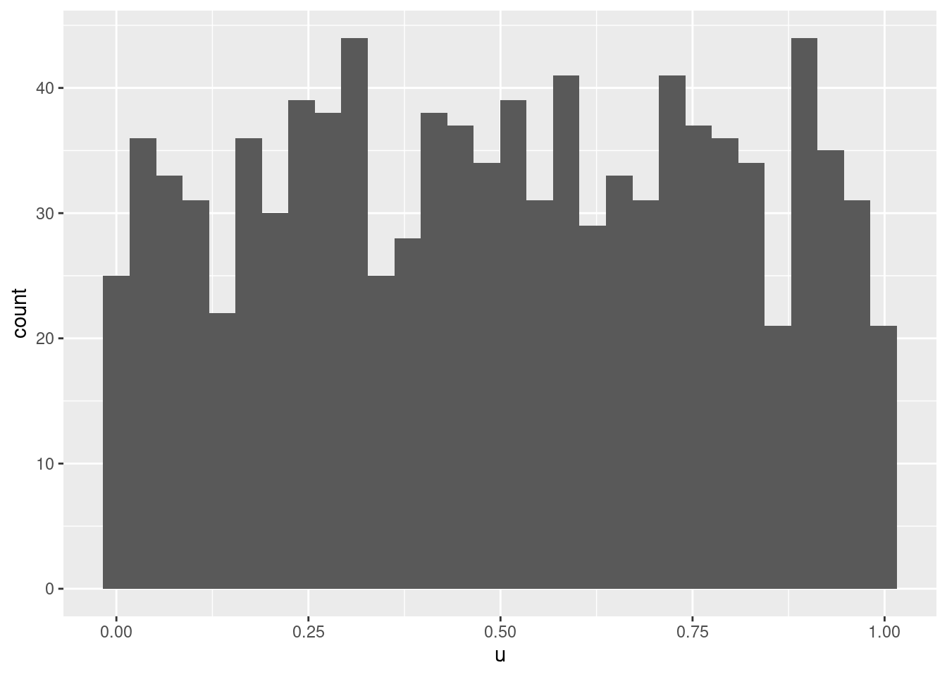

we obviously get random draws from the continuous uniform distribution $U[0,1]$, ie. $F(X)\sim\text{U}(0,1)$.

Now all we need to do is to solve this equation:

\[ F(X)=Z, Z\sim U[0,1] \] with respect to $X$: \[ X=F^{-1}(Z), Z\sim U[0,1] \]

For application this means that as long as we can draw from a continuous uniform distribution, and as long as we can write down $F^{-1}$, we can generate random draws for $X$.

Inversion sampling:

generate numbers $u_1,\dots,u_n$ from the continuous uniform distribution $U[0,1]$
transform $x_k=F^{-1}(u_k)$

In R, $F^{-1}(u_k)$ is given as q....

u <- runif(5)
qnorm(p = u)

## [1] -1.9728444 -1.2169369 -2.2157531 -0.8150545  2.4262442

qweibull(p = u, shape = 1, scale = 1)

## [1] 0.02455568 0.11857422 0.01344418 0.23258871 4.87592939

qbinom(p = u, size = 10, prob = .5)

## [1] 2 3 2 4 9

6 Case study

6.1 Let’s invent a data generating machanism

Because of a drought in one year, trees grow less in this year in comparison to the preceding year. However, by differences in the availability to growth-ressources by different elevations at the same mountain range, this reduction is reversed above a certain elevation threshold.

(elev <- seq(400, 1800, by = 50) / 1000)

##  [1] 0.40 0.45 0.50 0.55 0.60 0.65 0.70 0.75 0.80 0.85 0.90 0.95 1.00 1.05 1.10
## [16] 1.15 1.20 1.25 1.30 1.35 1.40 1.45 1.50 1.55 1.60 1.65 1.70 1.75 1.80

For species A and B:

muA <- .7 + .25 * elev
muB <- .8 + .15 * elev
paint <- colorspace::qualitative_hcl(n = 2)
ggplot(data = data.frame(k = rep(LETTERS[1:2], each = length(elev)), 
                         mu = c(muA, muB), 
                         elevation = c(elev, elev))) + 
  geom_line(aes(x = elevation, y = mu, color = k, group = k))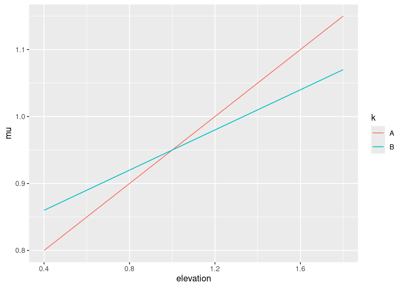

Random variation in site-specific availability to growth-ressources:

set.seed(123)
epsA <- rnorm(length(muA), sd = .05)
epsB <- rnorm(length(muB), sd = .05)
ggplot(data = data.frame(k = rep(LETTERS[1:2], each = length(elev)), 
                         y = c(muA + epsA, muB + epsB), 
                         elevation = c(elev, elev))) + 
  geom_point(aes(x = elevation, y = y, color = k, group = k))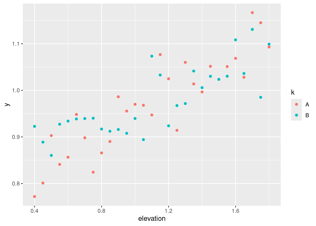

Compose outcome measurements y:

yA <- muA + epsA
yB <- muB + epsB

6.2 Introduction `formula`

formula notation for the data generating mechanism:

frmlaA <- as.formula(yA ~ elev)
str(frmlaA)

## Class 'formula'  language yA ~ elev
##   ..- attr(*, ".Environment")=<environment: R_GlobalEnv>

summary(frmlaA)

##  Length   Class    Mode 
##       3 formula    call

frmlaA[1]

## `~`()

frmlaA[2]

## yA()

frmlaA[3]

## elev()

yA and yB are measured outcomes, written on the left hand side of the formula
The left hand side is separated from the right hand side by ~
The right hand side expresses the explanatory variables that are either experimentally controlled, or – similar to the outcome – observed / measured. In our formula examples, elev is the only explanatory variable.
The parameters used for generating the outcome, .7, .25 and .05 for A, and .8, .15 and .05 for B, are not stated in the formula. Why? … because in real world applications, we don’t artificially invent, but rather want to estimate their plausible values based on our data.
Let’s assume it comes to our mind that a normal distribution is a statistical model that is quite useful to express the effects of variation in site-specific availability to growth-ressources on the outcome. Then:

We can use a formula directly for plot:

frmlaB <- as.formula(yB ~ elev)
plot(frmlaA, pch = "A", col = paint[1])
points(frmlaB, pch = "B", col = paint[2])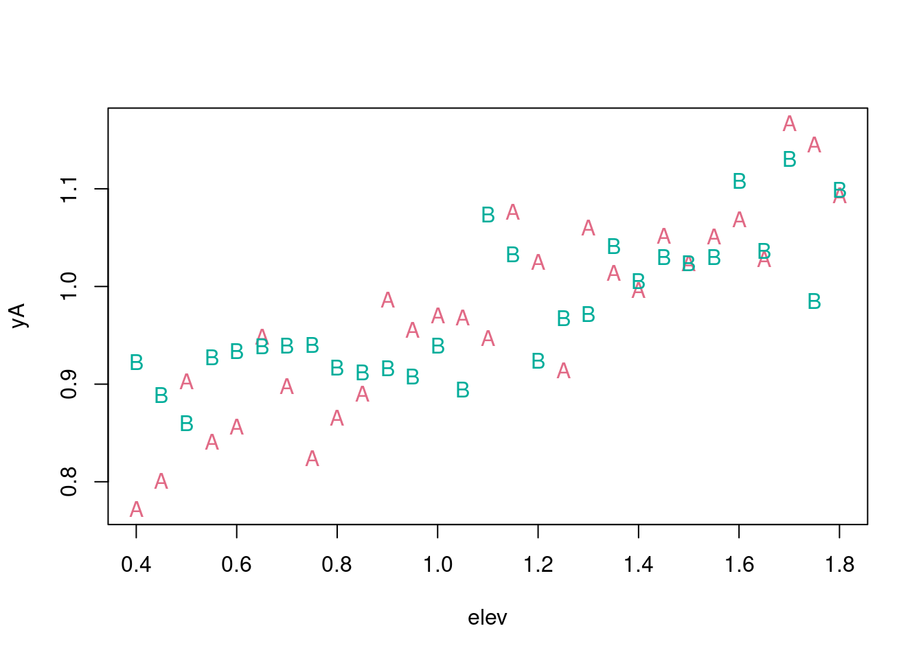

6.2.1 Using `formula` inside `lm`

mA <- lm(frmlaA)
mB <- lm(frmlaB)
par(mfrow = c(1, 2))
plot(frmlaA, pch = "A", col = paint[1])
abline(mA, col = paint[1])
points(frmlaB, pch = "B", col = paint[2])
abline(mB, col = paint[2])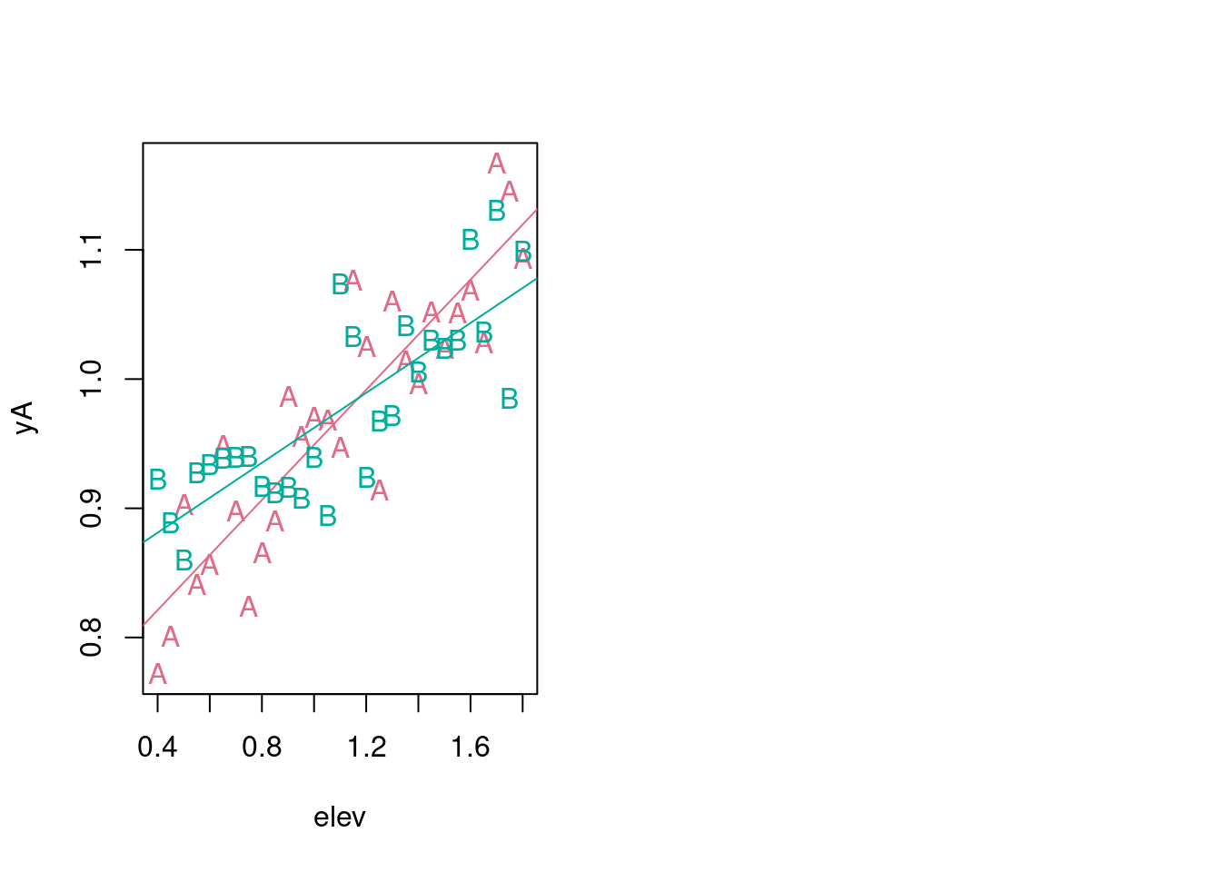

The data-generating mechanisms varied for varying species A, and B. Can we unify this into one description of a data-generating mechanism?

\[ yA=0.7+0.25\cdot\text{elev}+\texttt{rnorm(n=1, mu = 0, sd = .05)}\\ yB=0.8+0.15\cdot\text{elev}+\texttt{rnorm(n=1, mu = 0, sd = .05)}\\ \rightarrow y= 0.7+0.25\cdot\text{elev}+\texttt{(species == B)}\cdot(0.1-0.1\cdot\text{elev})+\texttt{rnorm(n=1, mu = 0, sd = .05)} \]

dfsim <- data.frame(y = c(yA, yB),
                    elev = c(elev, elev),
                    species = as.factor(rep(LETTERS[1:2], each = length(elev))))
dfsim$x <- dfsim$elev
## See: ?formula
frmla <- as.formula(y ~ x * species)
summary(frmla)

##  Length   Class    Mode 
##       3 formula    call

head(model.matrix(object = frmla, data = subset(dfsim, species == "A")))

##   (Intercept)    x speciesB x:speciesB
## 1           1 0.40        0          0
## 2           1 0.45        0          0
## 3           1 0.50        0          0
## 4           1 0.55        0          0
## 5           1 0.60        0          0
## 6           1 0.65        0          0

head(model.matrix(object = frmla, data = subset(dfsim, species == "B")))

##    (Intercept)    x speciesB x:speciesB
## 30           1 0.40        1       0.40
## 31           1 0.45        1       0.45
## 32           1 0.50        1       0.50
## 33           1 0.55        1       0.55
## 34           1 0.60        1       0.60
## 35           1 0.65        1       0.65

m <- lm(frmla, data = dfsim)
coef(m)

## (Intercept)           x    speciesB  x:speciesB 
##  0.73593782  0.21314912  0.09105386 -0.07786856

6.3 Inspection of estimated parameters

library("arm")

## Lade nötiges Paket: MASS

## 
## Attache Paket: 'MASS'

## Das folgende Objekt ist maskiert 'package:spatstat.geom':
## 
##     area

## Lade nötiges Paket: Matrix

## 
## Attache Paket: 'Matrix'

## Das folgende Objekt ist maskiert 'package:lmfor':
## 
##     updown

## Lade nötiges Paket: lme4

## 
## Attache Paket: 'lme4'

## Das folgende Objekt ist maskiert 'package:nlme':
## 
##     lmList

## 
## arm (Version 1.14-4, built: 2024-4-1)

## Working directory is /home/hsennhenn/Dropbox/Schreibtisch/oer_introduction_to_R_2024

## 
## Attache Paket: 'arm'

## Das folgende Objekt ist maskiert 'package:spatstat.geom':
## 
##     rescale

tmp <- sim(m)
B <- cbind(tmp@coef, tmp@sigma)
colnames(B)[ncol(B)] <- "sigma"
df_draws <- data.frame("k" = factor(rep(colnames(B), each = nrow(B)), levels = colnames(B)), 
                       "value" = as.numeric(B))
ggplot(data = df_draws, aes(x = k, y = value)) + 
  geom_boxplot()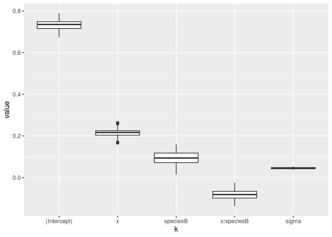

6.4 Predictive check

For only one data-point:

elev <- 1300 / 1000
species <- factor(c("A"), levels = levels(dfsim$species))
X <- model.matrix(frmla[-2], data = data.frame(x = elev, species = species))
X %*% B[1, -ncol(B)]

##       [,1]
## 1 1.015346

rnorm(n = 100, mean = X %*% B[1, -ncol(B)], sd = B[1, ncol(B)])

##   [1] 0.9899480 1.1019713 1.0041147 1.0777084 1.0207939 1.0035805 1.0309227
##   [8] 0.9790030 1.0654185 0.9655213 1.0515324 1.0261213 1.0216022 1.0481515
##  [15] 0.9765463 0.9598976 1.0021634 1.0701242 1.0414169 1.1183507 0.9699917
##  [22] 1.0201318 1.1534332 1.0162380 1.0556141 1.0537146 1.0881090 1.0178440
##  [29] 1.0697926 0.9364685 0.9813849 1.0188523 0.9886918 1.0254739 0.9378543
##  [36] 1.0395219 0.9930987 0.9944408 1.0085548 0.9889237 0.9373617 1.0426293
##  [43] 1.0165602 0.8777181 1.0653720 0.9841040 1.0241862 1.0285470 0.9678332
##  [50] 0.9471550 1.0845774 1.1022373 1.0423772 1.0228742 1.0215433 1.0295161
##  [57] 1.0029881 1.0627028 1.0466847 0.9884676 1.0209400 1.0170410 1.0183230
##  [64] 1.0617957 0.9920905 1.0434989 1.0232035 1.0137752 1.0596489 1.0216063
##  [71] 0.9658334 0.9573625 0.9998750 0.9829873 0.9593663 0.9856021 0.9328536
##  [78] 0.9964383 0.9988052 1.0020665 1.0143018 1.0317154 0.9942652 1.0288297
##  [85] 0.9723134 1.0454983 1.0192867 1.0104133 0.9847446 1.0920802 1.0327738
##  [92] 1.0264920 0.8984973 0.9266750 1.0125771 1.0557838 1.0140788 0.9701887
##  [99] 1.0081371 0.9915109

For the full data-frame:

X <- model.matrix(frmla[-2], data = dfsim)
head(X %*% B[1, -ncol(B)])

##        [,1]
## 1 0.8222726
## 2 0.8329990
## 3 0.8437253
## 4 0.8544516
## 5 0.8651779
## 6 0.8759042

dim(X %*% B[1, -ncol(B)])

## [1] 58  1

Ytilde <- matrix(nrow = nrow(B), ncol = nrow(dfsim), NA)
for (s in 1:nrow(B)) {
  tmp <- X %*% B[s, -ncol(B)]
  for (i in 1:nrow(dfsim)) {
    Ytilde[s, i] <- rnorm(n = 1, mean = tmp[i, 1], sd = B[s, ncol(B)])
  }
}
tmp <- apply(Ytilde, MAR = 1, FUN = density)
plot(0, 0, ylim = c(0, max(sapply(tmp, FUN = function(x){return(max(x$y))}))), 
     xlim = c(min(sapply(tmp, FUN = function(x){return(min(x$x))})), 
              max(sapply(tmp, FUN = function(x){return(max(x$x))}))), 
     type = "n", bty = "n", las = 1, xlab = "y", ylab = "(Predictive) Density")
invisible(sapply(tmp, FUN = lines, col = colorspace::sequential_hcl(n = 1, alpha = .1)))
lines(density(dfsim$y), lwd = 4)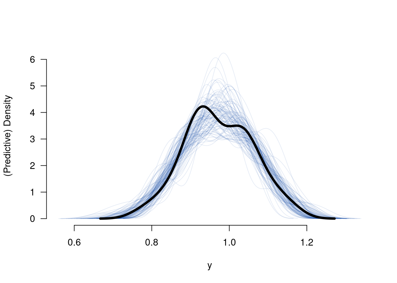

6.5 Model component `mu`

elev <- rep(c(400, 1800), 2) / 1000
species <- factor(rep(LETTERS[1:2], each = 2), levels = levels(dfsim$species))
(X <- model.matrix(frmla[-2], data = data.frame(x = elev, species = species)))

##   (Intercept)   x speciesB x:speciesB
## 1           1 0.4        0        0.0
## 2           1 1.8        0        0.0
## 3           1 0.4        1        0.4
## 4           1 1.8        1        1.8
## attr(,"assign")
## [1] 0 1 2 3
## attr(,"contrasts")
## attr(,"contrasts")$species
## [1] "contr.treatment"

Mu <- matrix(nrow = nrow(B), ncol = nrow(X), NA)
for (s in 1:nrow(B)) {
  Mu[s, ] <- X %*% B[s, -ncol(B)]
}
paint <- colorspace::qualitative_hcl(n = 2, alpha = .1)
plot(range(elev), range(Mu), type = "n", las = 1, xlab = "Elev [m/1000]", 
     ylab = "Model component 'mu'", bty = "n")
for (s in 1:nrow(Mu)) {
  lines(range(elev), Mu[s, 1:2], col = paint[1])
  lines(range(elev), Mu[s, 3:4], col = paint[2])
}
lines(range(elev), .7 + .25 * range(elev), col = colorspace::qualitative_hcl(n = 2)[1], lwd = 4)
lines(range(elev), .8 + .15 * range(elev), col = colorspace::qualitative_hcl(n = 2)[2], lwd = 4)
lines(range(elev), coef(m)[1] + coef(m)[2] * range(elev), col = colorspace::qualitative_hcl(n = 2)[1], lwd = 4, lty = 2)
lines(range(elev), coef(m)[1] + coef(m)[3] + (coef(m)[2] + coef(m)[4]) * range(elev), 
      col = colorspace::qualitative_hcl(n = 2)[2], lwd = 4, lty = 2)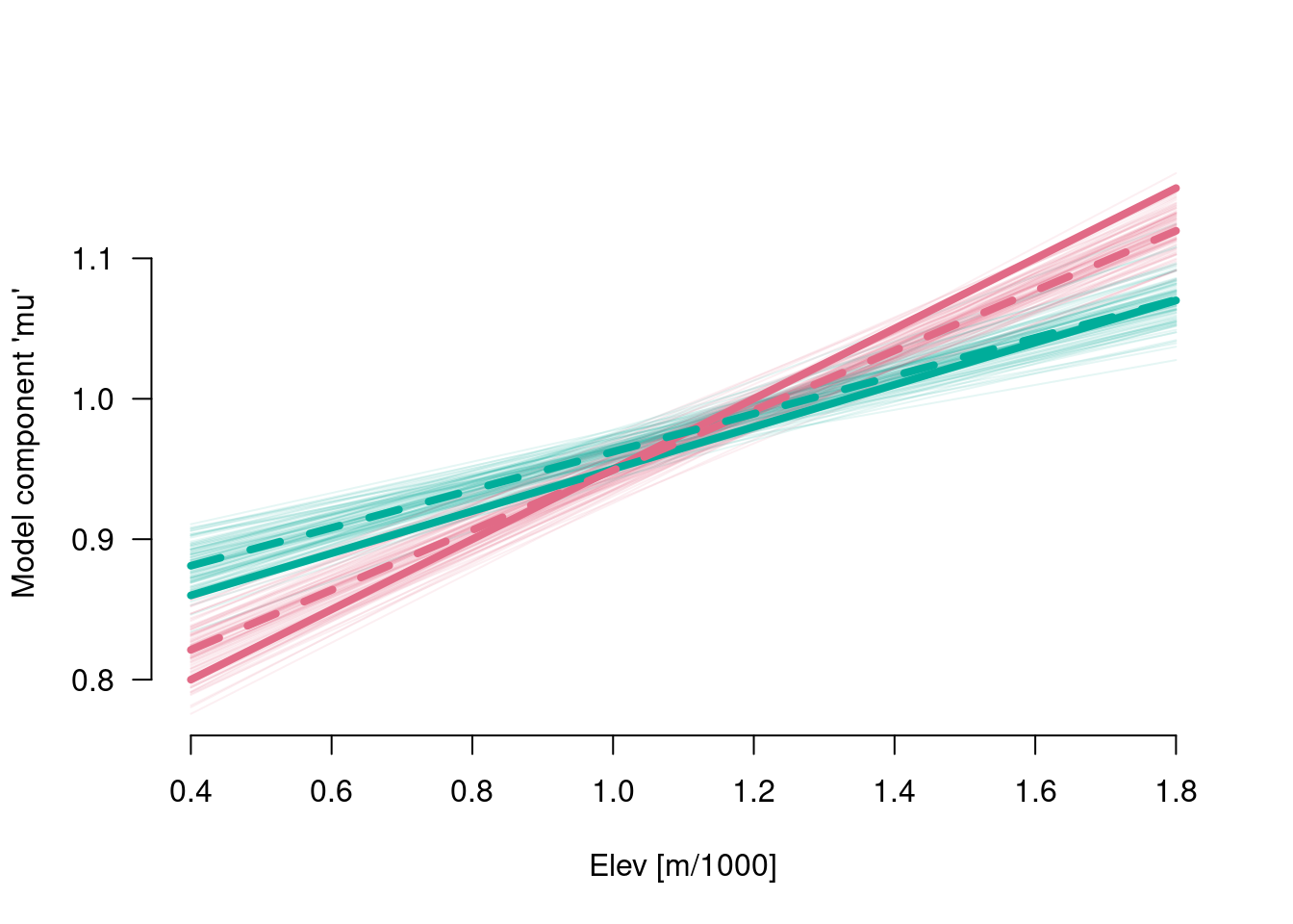

6.6 Real data

drought$x <- drought$elev / 1000
drought$y <- drought$bair
m <- lm(frmla, data = drought)
tmp <- sim(m)
B <- cbind(tmp@coef, tmp@sigma)

6.6.1 Predictive check

X <- model.matrix(frmla[-2], data = drought)
head(X %*% B[1, -ncol(B)])

##        [,1]
## 1 0.4047765
## 2 0.4672026
## 3 0.4771908
## 4 0.4946701
## 5 0.5071554
## 6 0.5620903

dim(X %*% B[1, -ncol(B)])

## [1] 34  1

Ytilde <- matrix(nrow = nrow(B), ncol = nrow(drought), NA)
for (s in 1:nrow(B)) {
  tmp <- X %*% B[s, -ncol(B)]
  for (i in 1:nrow(drought)) {
    Ytilde[s, i] <- rnorm(n = 1, mean = tmp[i, 1], sd = B[s, ncol(B)])
  }
}
tmp <- apply(Ytilde, MAR = 1, FUN = density)
plot(0, 0, ylim = c(0, max(sapply(tmp, FUN = function(x){return(max(x$y))}))), 
     xlim = c(min(sapply(tmp, FUN = function(x){return(min(x$x))})), 
              max(sapply(tmp, FUN = function(x){return(max(x$x))}))), 
     type = "n", bty = "n", las = 1, xlab = "y", ylab = "(Predictive) Density")
invisible(sapply(tmp, FUN = lines, col = colorspace::sequential_hcl(n = 1, alpha = .1)))
lines(density(drought$y), lwd = 4)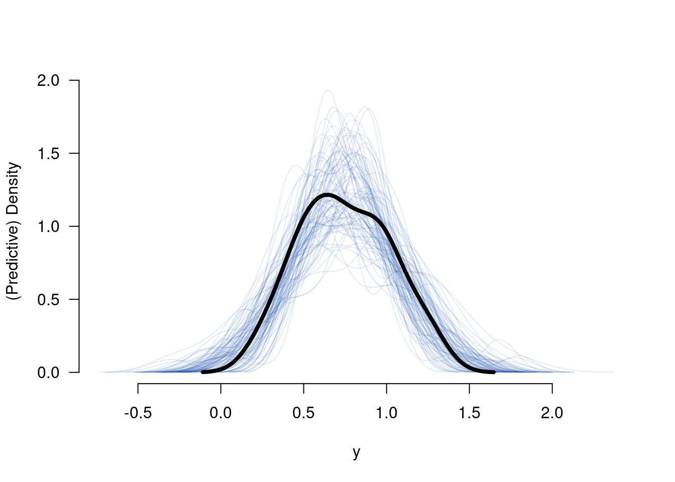

6.6.2 Model component `mu`

elev <- rep(c(400, 1800), 2) / 1000
species <- factor(rep(levels(drought$species), each = 2), levels = levels(drought$species))
(X <- model.matrix(frmla[-2], data = data.frame(x = elev, species = species)))

##   (Intercept)   x speciesSpruce x:speciesSpruce
## 1           1 0.4             0             0.0
## 2           1 1.8             0             0.0
## 3           1 0.4             1             0.4
## 4           1 1.8             1             1.8
## attr(,"assign")
## [1] 0 1 2 3
## attr(,"contrasts")
## attr(,"contrasts")$species
## [1] "contr.treatment"

Mu <- matrix(nrow = nrow(B), ncol = nrow(X), NA)
for (s in 1:nrow(B)) {
  Mu[s, ] <- X %*% B[s, -ncol(B)]
}
paint <- colorspace::qualitative_hcl(n = 2, alpha = .1)
plot(range(elev), range(Mu), type = "n", las = 1, xlab = "Elevation [m/1000]", 
     ylab = "Model component 'mu'", bty = "n")
for (s in 1:nrow(Mu)) {
  lines(range(elev), Mu[s, 1:2], col = paint[1])
  lines(range(elev), Mu[s, 3:4], col = paint[2])
}
lines(range(elev), coef(m)[1] + coef(m)[2] * range(elev), col = colorspace::qualitative_hcl(n = 2)[1], lwd = 4, lty = 2)
lines(range(elev), coef(m)[1] + coef(m)[3] + (coef(m)[2] + coef(m)[4]) * range(elev), 
      col = colorspace::qualitative_hcl(n = 2)[2], lwd = 4, lty = 2)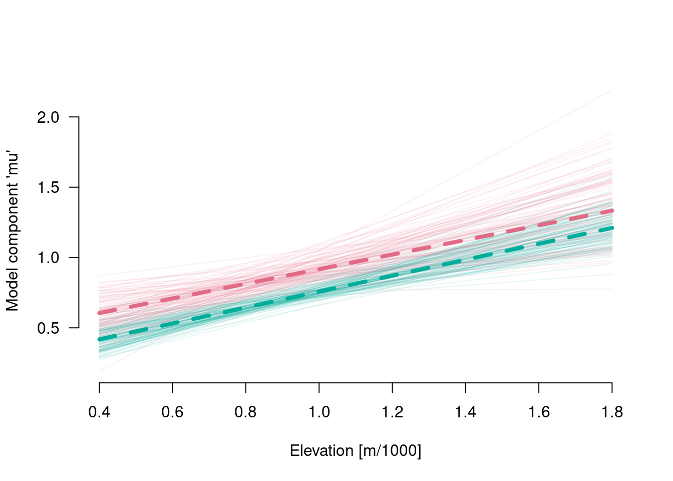

References

Private webpage: uncertaintree.github.io ↩︎

Introduction to R: Session 04