All contents are licensed under CC BY-NC-ND 4.0.

1 R markdown

R markdown (Allaire et al. (2021), Xie, Allaire, and Grolemund (2018), Xie, Dervieux, and Riederer (2020)) offers an environment to combine the analysis / manipulation / … of data with an immediate production of a document in one step (all materials of this course were created with a variant of R markdown).

With a single R markdown file, you can:

save an evaluate R code, and
generate a report (article, presentation slides, …) containing the results of the evaluation of the R code.

R markdown documents are completely reproducible and support a variety of static and dynamic output formats (docx, pdf, html, …).

1.1 Structure

An R markdown file is essentially divided into three areas:

Title:

---
title: "Estimating Potential for Late-Frost-Events in Goettingen"
author: "Holger Sennhenn-Reulen"
date: "June 26, 2024"
output: word_document
---

R code ‘chunks’:

```{r}
summary(frost)
```

and, embedded in between, text with (reduced) formatting:

This sentence will be given as ordinary text in the output document, 
with words in *italics* or **bold**.

1.2 Installation

A connection to the internet is required for the following steps:

Create a new folder markdown files in your favorite working directory.
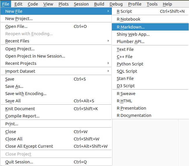
Start RStudio and click on File \(\rightarrow\) New File \(\rightarrow\) R Markdown:
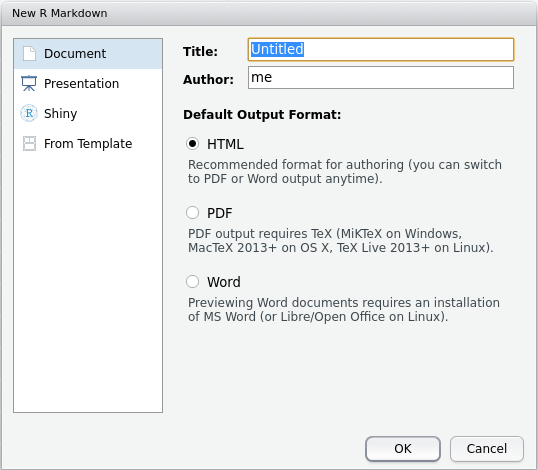
After clicking on ‘R Markdown’ you will be asked whether you want to install some R packages . After confirmation, with subsequent installation, the following window should open:
Enter a title and your name and mark the selection ‘Word’. Click on ‘OK’.
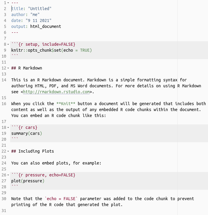
The following document is generated (in this example, the output is still set on the default html_document):
Save this file in the markdown files folder: The file has the extension.Rmd, for R-Markdown.
Finally: click on the blue ‘Knit’ button.
A Word / OpenOffice Writer file with R commands, graphics and results should open.

1.3 Links & misc

Get started!
R markdown cheat sheet
R markdown reference guide
Click Help \(\rightarrow\) Markdown Quick Reference
Inlcude template file:

output:
  word_document: 
    highlight: null
    toc: yes
    reference_docx: markdown_word_style_template.docx
---

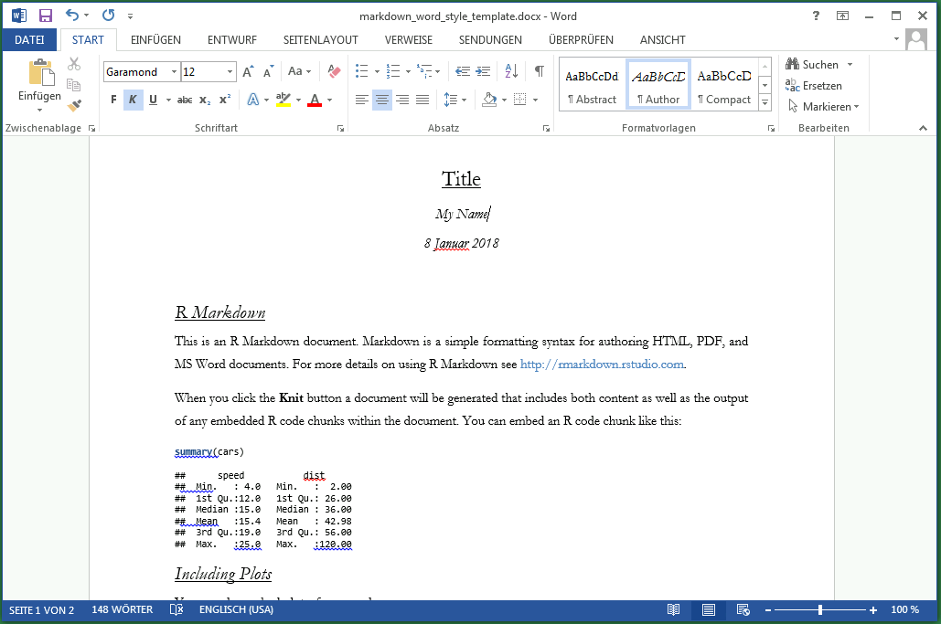
where markdown_word_style_template.docx is a file that stores built-in Microsoft Office Word styles (German: Formatvorlagen): Word template

2 Other topics

2.1 Citation

Give credit to package authors and maintainers by citing R packages:

citation("mgcv")

2.2 R-Code Structure

I usually use the following six sections structure for applied statistics on real data:

1st section: Organize R session (Load packages, set working directory, …)
2nd section: Data management (Load data, manipulate and organize data, hold your global environment clean using rm())
3rd section: Descriptive analysis (Plots, plots, plots, …)
4th section: Statistical modelling
5th section: Visualization (is better than tabulation) of results
6th section: Show the outcome of sessionInfo()

Note: If this is your markdown structure, then whatever you show in section 5 is fully reproducible (given you don’t make excessive use of save and load).

2.3 Dput

The R function dput(...) comes handy here and there:

dput(names(drought))

## c("bair", "elev", "species")

References

Allaire, JJ, Yihui Xie, Jonathan McPherson, Javier Luraschi, Kevin Ushey, Aron Atkins, Hadley Wickham, Joe Cheng, Winston Chang, and Richard Iannone. 2021. Rmarkdown: Dynamic Documents for r. https://github.com/rstudio/rmarkdown.

Xie, Yihui, J. J. Allaire, and Garrett Grolemund. 2018. R Markdown: The Definitive Guide. Boca Raton, Florida: Chapman; Hall/CRC. https://bookdown.org/yihui/rmarkdown.

Xie, Yihui, Christophe Dervieux, and Emily Riederer. 2020. R Markdown Cookbook. Boca Raton, Florida: Chapman; Hall/CRC. https://bookdown.org/yihui/rmarkdown-cookbook.

Private webpage: uncertaintree.github.io ↩︎

Introduction to R: Session 05