All contents are licensed under CC BY-NC-ND 4.0.

1 R markdown

R markdown (Allaire et al. (2021), Xie, Allaire, and Grolemund (2018), Xie, Dervieux, and Riederer (2020)) offers an environment to combine the analysis / manipulation / … of data with an immediate production of a document in one step (all materials of this course were created with a variant of R markdown).

With a single R markdown file, you can:

save an evaluate R code, and
generate a report (article, presentation slides, …) containing the results of the evaluation of the R code.

R markdown documents are completely reproducible and support a variety of static and dynamic output formats.

1.1 Structure

An R markdown file is essentially divided into three areas:

Title:

---
title: "Estimating Potential for Late-Frost-Events in Goettingen"
author: "Holger Sennhenn-Reulen"
date: "November 09, 2021"
output: word_document
---

R code ‘chunks’:

```{r}
summary(frost)
```

and, embedded in between, text with (reduced) formatting:

This sentence will be given as ordinary text in the output document, 
with words in *italics* or **bold**.

1.2 Installation

A connection to the internet is required for the following steps:

Create a new folder markdown files in your favorite working directory.
Start RStudio and click on File \(\rightarrow\) New File \(\rightarrow\) R Markdown: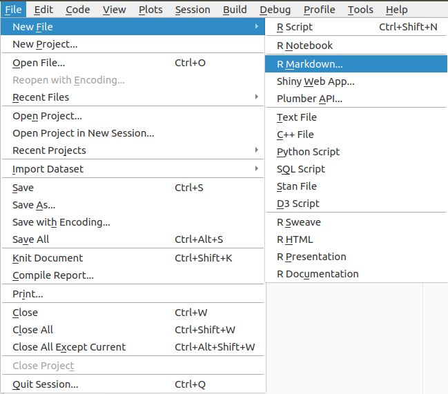
After clicking on ‘R Markdown’ you will be asked whether you want to install some R packages . After confirmation, with subsequent installation, the following window should open:
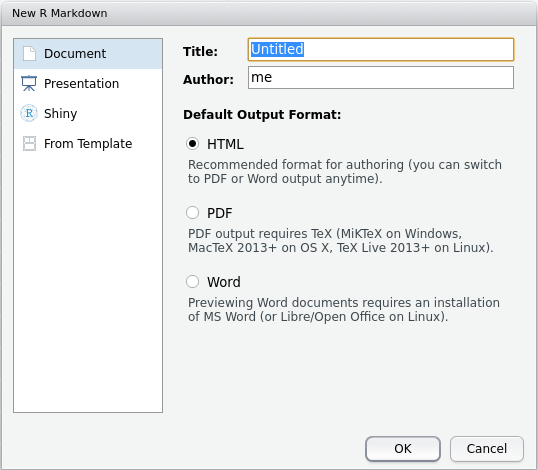
Enter a title and your name and mark the selection ‘Word’. Click on ‘OK’.
The following document is generated (in this example, the output is still set on the default html_document):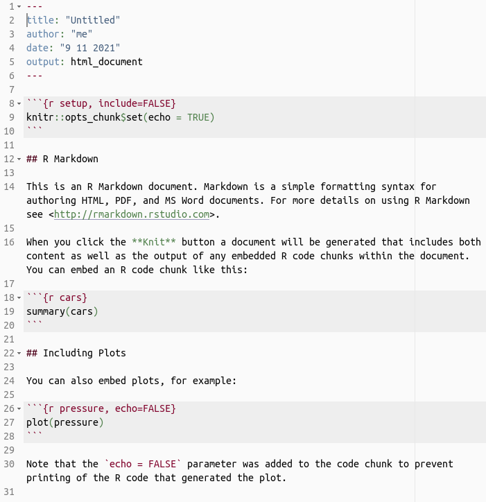
Save this file in the markdown files folder: The file has the extension.Rmd, for R-Markdown.
Finally: click on the ‘Knit’ button.
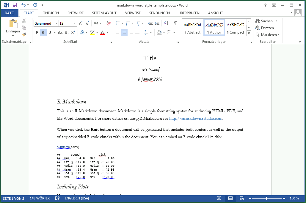
A Word / OpenOffice Writer file with R commands, graphics and results should open.

1.3 Links & misc

Get started!
R markdown cheat sheet
R markdown reference guide
Click Help \(\rightarrow\) Markdown Quick Reference
Inlcude template file:

output:
  word_document: 
    highlight: null
    toc: yes
    reference_docx: markdown_word_style_template.docx
---

where markdown_word_style_template.docx is a file that stores built-in Microsoft Office Word styles (German: Formatvorlagen): Word template

2 Other topics

Give credit to package authors and maintainers by citing R packages:

citation("mgcv")

Six sections structure for applied statistics on real data:
- 1st section: Organize R session (Load packages, set working directory, …)
- 2nd section: Data management (Load data, manipulate and organize data, hold your global environment clean using rm())
- 3rd section: Descriptive analysis (Plots, plots, plots, …)
- 4th section: Statistical modelling
- 5th section: Visualisation (is better than tabulation) of results
- 6th section: Show the outcome of sessionInfo()
- Note: If this is your markdown structure, then whatever you show in section 5 is fully reproducible (given you don’t make excessive use of save and load), and there is no better feeling than bycycle-commuting home through sunshine, knowing that your analysis is reproducible on the next day!
dput(...) comes handy here and there.

References

Allaire, JJ, Yihui Xie, Jonathan McPherson, Javier Luraschi, Kevin Ushey, Aron Atkins, Hadley Wickham, Joe Cheng, Winston Chang, and Richard Iannone. 2021. Rmarkdown: Dynamic Documents for R. https://github.com/rstudio/rmarkdown.

Xie, Yihui, J.J. Allaire, and Garrett Grolemund. 2018. R Markdown: The Definitive Guide. Boca Raton, Florida: Chapman; Hall/CRC. https://bookdown.org/yihui/rmarkdown.

Xie, Yihui, Christophe Dervieux, and Emily Riederer. 2020. R Markdown Cookbook. Boca Raton, Florida: Chapman; Hall/CRC. https://bookdown.org/yihui/rmarkdown-cookbook.

Private webpage: uncertaintree.github.io ↩

Introduction to R: Session 05